What are Loan Limits
Loan Limits are a policy design that assists in determining which single family residential mortgage loans are eligible for purchase, securitization and/or guarantee by the the U.S. Federal Government (FHA, VA, USDA) or Government Sponsored Enterprises (Fannie Mae and Freddie Mac).
if(!require(pacman)){
  install.packages("pacman")
  library(pacman)
}

p_load(tidyverse, lubridate, tidycensus, tigris, sf,
       scales, xfun, rio, janitor, rvest)

options(tigris_use_cache = TRUE)
Terminology for Loan Limits:
1. Conventional Loan Limits (CLLs): Fannie Mae and Freddie Mac eligible balance
2. Government Loan Limits):
+ FHA - Forward Mortgages, FHA - Home Equity Conversion Mortgages (reverse)
+ VA Loan Limits
Factors for determining loan limits:
1. Number of units in the home
2. Geography (national, state, county)
3. Annual home price appreciation
Then there are two types of Loan Limits:
* National baseline: Floor - Defined by Home Price Appreciation (HPA) estimates
* High Cost Area Limits: ceiling - 150% of baseline for areas with greater than 115% of median home price relative to baseline
* Between the Floor and the Ceiling
How are they set?
The Home and Economic Recovery Act (HERA) outlines by statute how the loan limits are determined. The respective covered government agencies then annually make available the limits for the following year.
The following years limits are normally published in November.
1. FHA
2. Federal Housing Finance Agency - regulator of Fannie Mae and Freddie Mac
For this post, we’ll specifically focus on: Conventional Loan Limits. Below we set a series of fixed values used for performing the calculations.
# Data source for Conforming loan limits: 2022 and 2021
ref_cll_url <- c(
  "https://www.fhfa.gov/DataTools/Downloads/Documents/Conforming-Loan-Limits/FullCountyLoanLimitList2022_HERA-BASED_FINAL_FLAT.xlsx",
  "https://www.fhfa.gov/DataTools/Downloads/Documents/Conforming-Loan-Limits/FullCountyLoanLimitList2021_HERA-BASED_FINAL_FLAT.xlsx"
)

# Home Price Index data from FHFA
fhfa_hpi_url <- "https://www.fhfa.gov/HPI_master.csv"

# FHFA Home Price Index (HPI) used to set Conventional Conforming Loan Limits
idx_of_interest <- "traditional - expanded-data"

# Published Base Loan Limits 2021, 2022
cll_base_2021 <- 548250.00
cll_base_2022 <- 647200.00
# Conditions of Loan Limit Ceiling
cll_limit_condition <- .15
cll_hca <- 1.5

# cll_med_2021 <- cll_base_2021/(1-cll_limit_condition)
# cll_med_2022 <- cll_base_2022/(1-cll_limit_condition)

# Ceiling value for each year
cll_hca_ceilinng_2021 <- cll_base_2021*cll_hca
cll_hca_ceiling_2022 <- cll_base_2022*cll_hca
Get the Data
Below we read in the data sets:
1. Geographic data for mapping at the end
2. Read in the conforming loan limits for both 2021 and 2022
3. Read in the FHFA Home Price Index which is used to determine the 2022 limits
For future use, we define a function for reading in the HPI data to include the year-over-year home price growth measure. The Q3 reported value is the measure utilized for purposes of estimating previous year home-price appreciation that informs the following year levels.
d_sf_geo <- get_acs(geography = "county", variables = c(hinc = "B19013_001"),
                    geometry = T, survey = "acs5", year = 2019,
                    resolution = "20m")%>%
  tigris::shift_geometry()

d_sf_state <- get_acs(geography = "state", variables = c(hinc = "B19013_001"),
                      geometry = T, survey = "acs5", year = 2019,
                      resolution = "20m")%>%
  tigris::shift_geometry()
# Get 2 most recent years of limits (2021, 2022)
d_in_cll <- map_df(ref_cll_url,
                ~rio::import(file = .x, ), .id = "fname")%>%
  setNames(., .[1,])%>%
  .[-1,]%>%
  clean_names(.)%>%
  mutate_if(is.character, ~str_trim(., side = "both"))%>%
  # mutate_at(.vars = vars(ends_with("unit_limit")), funs(as.double(.)))%>%
  mutate(yr_cll = ifelse(x1==1, 2022, 2021),
         fips_state_code = ifelse(is.na(fips_state_code), na, fips_state_code))%>%
  filter(str_length(fips_state_code) == 2)%>%
  select(-c(na,x1))%>%
  rename(state_name = state, cbsa_code = cbsa_number)%>%
  pivot_longer(one_unit_limit:four_unit_limit, names_to = "hunit_num",
               values_to = "cll_amt_limit")%>%
  relocate(yr_cll, .before = fips_state_code)%>%
  mutate(cll_amt_limit = str_trim(cll_amt_limit, side = "both")%>%
           str_replace_all(., "[^[0-9]]", "")%>%
           as.numeric(),
         hunit_num = case_when(
           hunit_num == "one_unit_limit" ~ 1,
           hunit_num == "two_unit_limit" ~ 2,
           hunit_num == "three_unit_limit" ~ 3,
           TRUE ~ 4))

# Read in FHFA HPI data

d_in_hpi <- read_csv(fhfa_hpi_url)%>%
  mutate(
    period_mo = case_when(
      period == 2 ~ 4,
      period == 3 ~ 7,
      period == 4 ~ 10,
      TRUE ~ period),
    dt_full = ymd(paste(yr, period_mo, "01", sep = "-")),
    hpi_type_new = paste(hpi_type, hpi_flavor, sep = " - "))

# Function to calculate home price appreciation (HPA) for national baseline (floor)


# f_get_cll_hpa <- function(df_in=NULL,fhfa_hpi_index = NULL,
#                           dt_hpi_reported = NULL){
#   dt_hpi_reported <- dt_hpi_reported%>%ymd(.)
#   dt_prev_hpi <- (lubridate::ymd(dt_hpi_reported) - lubridate::years(1))
#
#   t_ref <- df_in%>%
#     filter(place_id == "USA")%>%
#     filter(hpi_type_new == fhfa_hpi_index)%>%
#     filter(dt_full %in% c(dt_hpi_reported, dt_prev_hpi))%>%
#     select(hpi_type_new, dt_full, index_sa)%>%
#     arrange(dt_full)%>%
#     mutate(sa_hpa12_2022 = (index_sa/lag(index_sa,1))-1)
#
#   v_hpa_factor <- t_ref%>%
#     na.omit()%>%
#     select(sa_hpa12_2022)%>%
#     pull(.)%>%
#     as.numeric()
#
#   # Verify if it is accurate
#   check_calc <- cll_base_2021 * (1+v_hpa_factor)
#   print(paste("expected: ", cll_base_2022))
#   print(paste("calc result: ", check_calc))
#   print(paste("statute indicates, round to the nearest $25th"))
# }
Home Price Index
# Ge most recent HPI reported values for annotating our plot
most_recent <- d_in_hpi%>%
  filter(place_id == "USA")%>%
  select(hpi_type_new, dt_full, index_nsa, index_sa)%>%
  group_by(hpi_type_new)%>%
  mutate(sa_hpa12 = (index_sa/lag(index_sa,4))-1,
         nsa_hpa12 = (index_nsa/lag(index_nsa,4))-1)%>%
  slice(which.max(dt_full))

# Get a subset of data for relevant time series
d_hpa <- d_in_hpi%>%
  filter(hpi_type_new ==idx_of_interest)%>%
  filter(year(dt_full) > 2000)%>%
  filter(place_id == "USA")%>%
  select(hpi_type_new, dt_full, index_nsa, index_sa)%>%
  arrange(dt_full)%>%
  mutate(sa_hpa12 = (index_sa/lag(index_sa,4))-1)


# Plot raw index values
p1_hpa <- d_hpa%>%
  ggplot()+
  geom_line(aes(x = dt_full, y = index_sa), size = 1.15)+
  geom_point(data = filter(most_recent, hpi_type_new == idx_of_interest),
             aes(x = dt_full, y = index_sa),
             size = 3.25, color = "dodgerblue", alpha = .8)+
  geom_text(data = filter(most_recent, hpi_type_new == idx_of_interest),
            aes(x = dt_full-years(1), y = index_sa,
                label = round(index_sa, 2)))+
  scale_y_continuous(breaks = c(seq(0,375, 25)), limits = c(0,375) )+
  labs(title = "FHFA HPI - Expanded Data, Raw Index Value",
       subtitle = "U.S., Q3-2021",
       y = "Index, Seasonally Adjusted (SA)",
       x = NULL)+
  theme_minimal()+
  theme(axis.line.x = element_blank(),
        panel.grid.major.y = element_blank())

# Plot year-over-year percent change

p2_hpa <- d_hpa%>%
  ggplot()+
  geom_line(aes(x = dt_full, y = sa_hpa12), size = 1.15)+
  geom_hline(yintercept = 0)+
  geom_point(data = filter(most_recent, hpi_type_new == idx_of_interest),
             aes(x = dt_full, y = sa_hpa12),
             size = 3.25, color = "dodgerblue", alpha = .8)+
  geom_text(data = filter(most_recent, hpi_type_new == idx_of_interest),
            aes(x = dt_full-years(1), y = sa_hpa12,
                label = paste0(round(sa_hpa12*100, 4), "%")))+
  scale_y_continuous(breaks = c(seq(-.2, .25, .05)), limits = c(-0.2,.25),
                     labels = function(x) paste0(round(x*100, 2), "%"))+
  labs(title = "FHFA HPI - Expanded Data, Year-Over-Year % Change",
       subtitle = "U.S., Q3-2021",
       y = "Index, Seasonally Adjusted (SA)",
       x = NULL)+
  theme_minimal()+
  theme(axis.line.x = element_blank(),
        panel.grid.major.y = element_blank())

p1_hpa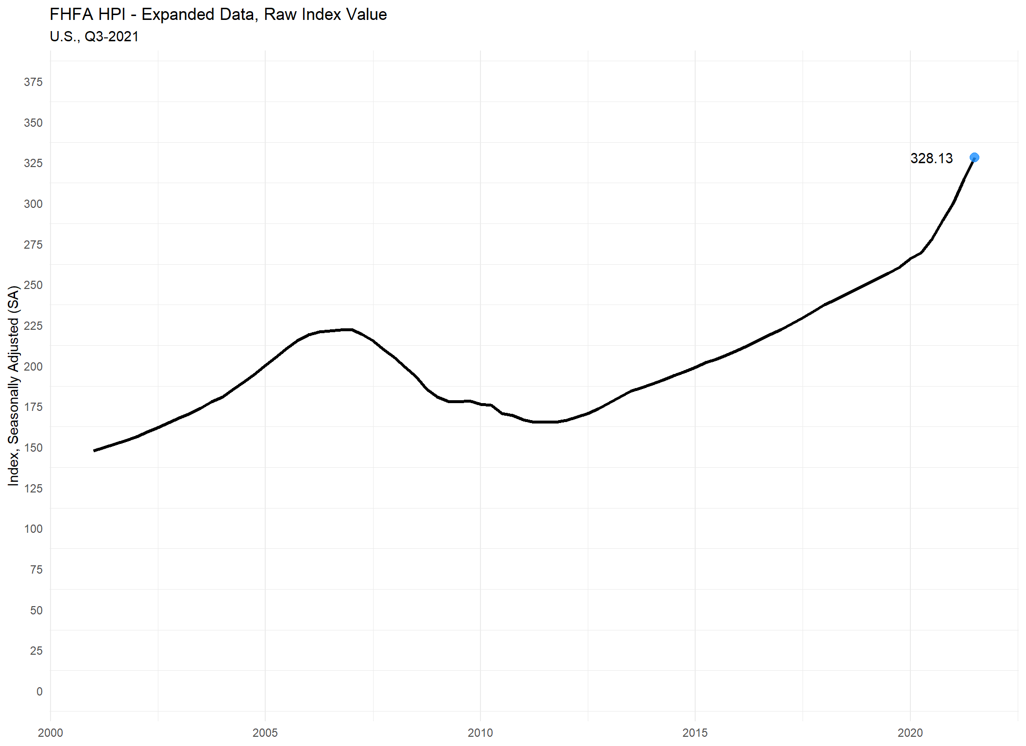
p2_hpa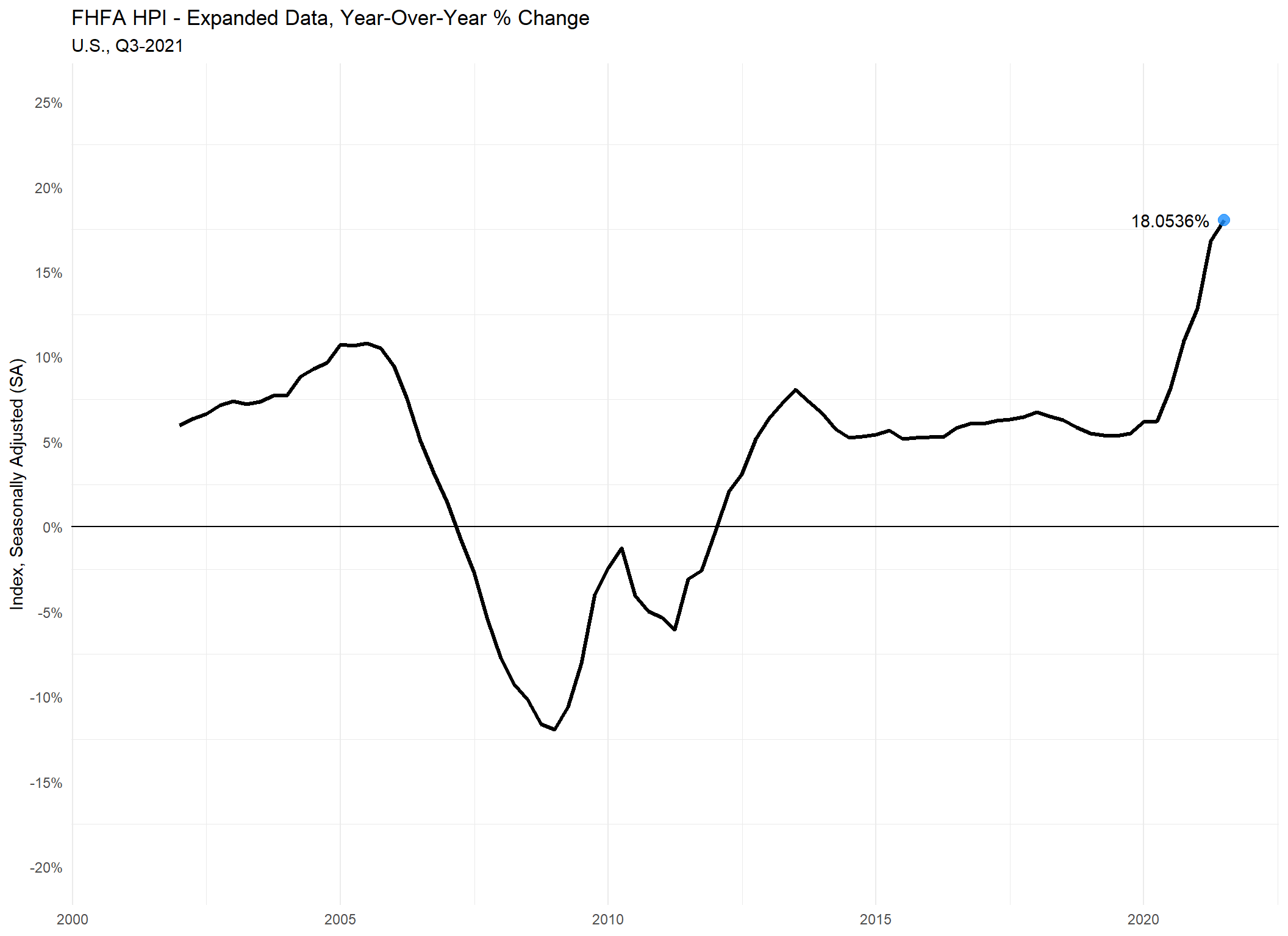
Conforming Loan Limits
# Create subsest of Conforming Loan Limits
d_cll_sfr_2022 <- d_in_cll%>%
  filter(hunit_num == 1)%>%
  filter(yr_cll == 2022)%>%
  mutate(fips5 = paste0(fips_state_code, fips_county_code))%>%
  select(yr_cll, fips5, hunit_num, ends_with("_name"), cll_amt_limit)%>%
  mutate(cll_type = case_when(
    cll_amt_limit == cll_base_2022 ~ "Base-Floor",
    cll_amt_limit > cll_base_2022 & cll_amt_limit < cll_hca_ceiling_2022 ~ "Between",
    cll_amt_limit == cll_hca_ceiling_2022 ~ "Ceiling"
  ))

# Create a 2021 v. 2022 table
d_cll_compare <- d_in_cll%>%
  filter(hunit_num == 1)%>%
  filter(yr_cll == 2021)%>%
  mutate(fips5 = paste0(fips_state_code, fips_county_code))%>%
  select(fips5, county_name, state_name, cll_2021 = cll_amt_limit)%>%
  left_join(., d_in_cll%>%
              filter(hunit_num == 1)%>%
              filter(yr_cll == 2022)%>%
              mutate(fips5 = paste0(fips_state_code, fips_county_code))%>%
              select(fips5, cll_2022 = cll_amt_limit))%>%
  mutate(raw_diff = cll_2022-cll_2021,
         pct_limit_chng = ((cll_2022/cll_2021)-1))

# Create a summary of 2022 CLL "Types"
t1_cll <- d_cll_sfr_2022%>%
  group_by(cll_type)%>%
  summarize(cnt = n())%>%
  knitr::kable()

# Map all U.S. Counties, filling based on Conforming Loan Limit Type
m1_cll <- d_sf_geo%>%
  geo_join(., d_cll_sfr_2022, by_sp = "GEOID", by_df = "fips5")%>%
  st_set_crs(st_crs(d_sf_geo))%>%
  ggplot()+
  geom_sf(aes(fill = cll_type), color = "white", lwd = .1, alpha = .8)+
  geom_sf(data = d_sf_state, fill = NA, lwd = 0.7, color = "black")+
  scale_fill_viridis_d("")+
  labs(title = "Conforming Loan Limits (Conventional)",
       subtitle = "As of 2022")+
  theme_void()+
  theme(legend.position = "bottom")

t1_cll | cll_type | cnt |
|---|---|
| Base-Floor | 3074 |
| Between | 57 |
| Ceiling | 102 |
m1_cll