TidyTuesday - Kenya & Italy Population by Age Cohort

Read-in Tidy Tuesday Kenya population by age data

d_pop_kenya_cnty <- rKenyaCensus::V3_T2.3%>%
  filter(grepl(Age, pattern = "\\-", ignore.case = T)==F)%>%
  filter(Age != "Total")%>%
  filter(Age != "Not Stated")%>%
  group_by(County)%>%
  filter(SubCounty == "ALL")%>%
  ungroup()%>%
  mutate(Age = Age%>%as.numeric())%>%
  filter(Age < 85 & Age > 16)%>%
  mutate(age_cut = cut(Age%>%as.numeric(), breaks = c(seq(0,85,5), Inf)))%>%
  separate(age_cut, sep = ",", into = c("from", "to"), remove = F)%>%
  mutate_at(vars("from", "to"), str_replace_all, pattern = "[^0-9]","")%>%
  mutate(to = as.numeric(to)-1)%>%
  mutate(clean_lab = paste0(from, " - ", as.character(to)), 
         clean_lab = if_else(grepl(clean_lab, pattern = "NA")==T, "85+", clean_lab))%>%
  select(-c(from, to, SubCounty, Age))%>%
  group_by(County, age_cut)%>%
  filter(row_number() == 1)%>%
  mutate(tot_pop = sum(Total, na.rm = T), 
         female_pct = round(sum(Female, na.rm = T)/tot_pop,2), 
         male_pct = round(sum(Male, na.rm = T)/tot_pop, 2))%>%
  ungroup()

d_prop_total <- d_pop_kenya_cnty%>%
  select(County, age_cut, clean_lab, Male, Female)%>%
  pivot_longer(., cols = -c("County", "age_cut", "clean_lab"),
               names_to = "sex", 
               values_to = "value")%>%
  mutate(tot_pop = sum(value, na.rm = T))%>%
  group_by(age_cut, clean_lab, sex, .add = T)%>%
  summarize(cohort_pop = sum(value, na.rm = T), 
            pct_tot = cohort_pop/unique(tot_pop))%>%
  mutate(plot_value_pct = if_else(sex=="Male", round((pct_tot*-1)*100,2), 
                                  round(pct_tot*100, 2)))%>%
  arrange(age_cut)%>%
  ungroup()

Plot Kenya population pyramid by age distribution and gender

ggplot(data = d_prop_total%>%arrange(desc(age_cut)),
       aes(x = age_cut, y = plot_value_pct, fill = sex))+ 
  geom_bar(stat = "identity", width = 1, color = "white")+
  theme_minimal(base_family = "Roboto") + 
  scale_y_continuous(breaks = c(seq(-10, 10, 1)), labels = function(y) paste0(abs(y), "%"))+ 
  scale_x_discrete(labels = unique(d_prop_total$clean_lab)) + 
  scale_fill_manual(name = "Kenya", values = c("royalblue4", "royalblue1")) + 
  coord_flip() + 
  labs(x = "", 
       y = "", 
       title = "Kenya Age Pyramid", 
       subtitle = "Population by sex and age group, 2019, % of Total", 
       fill = "", 
       caption = "Source: Shelmith Kariuki (2020). \n
       rKenyaCensus: 2019 Kenya Population and Housing Census Results. R package version 0.0.2")+
  dark_theme_minimal()+
  theme(legend.position = "top", 
        legend.direction = "horizontal")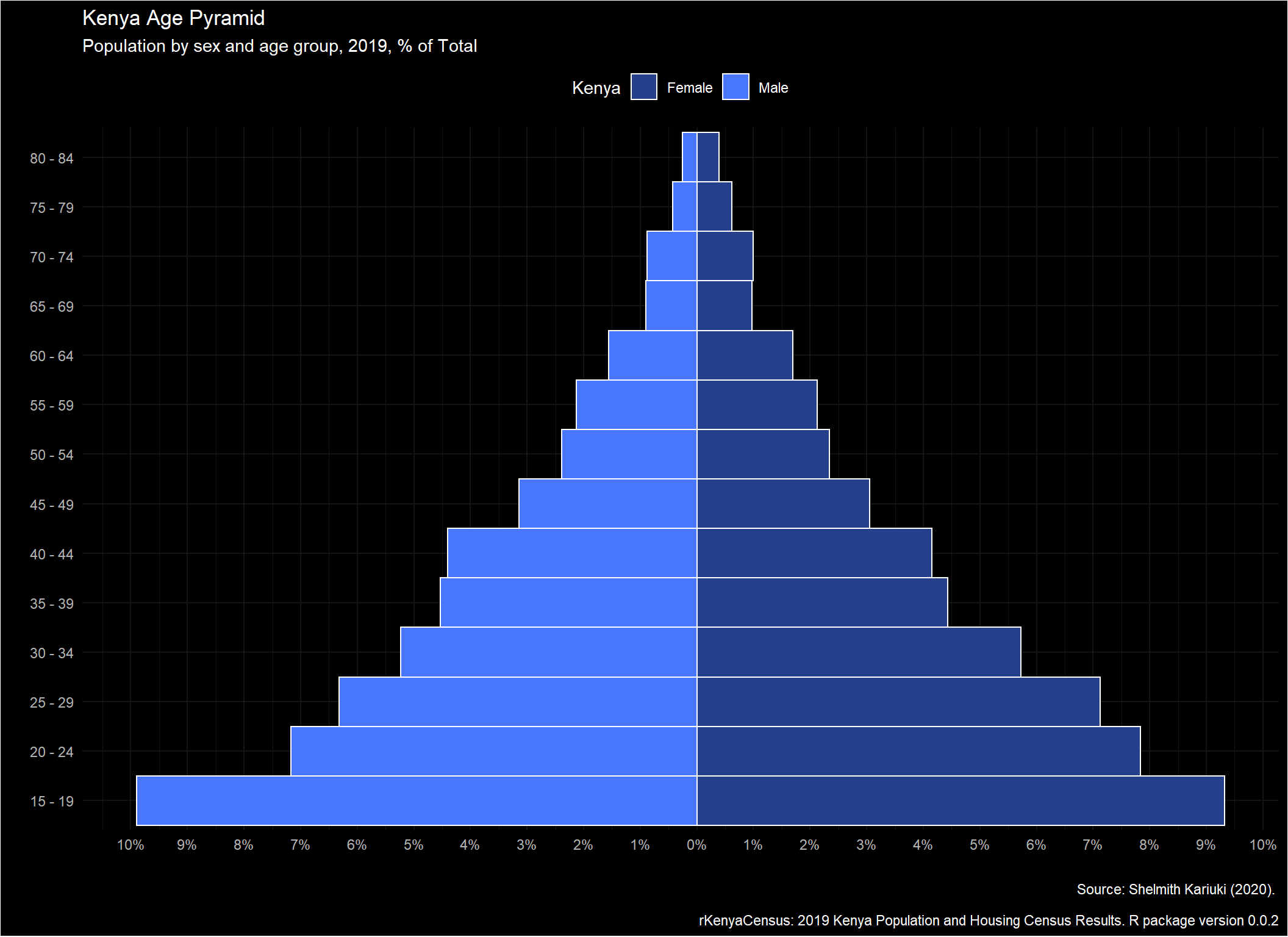

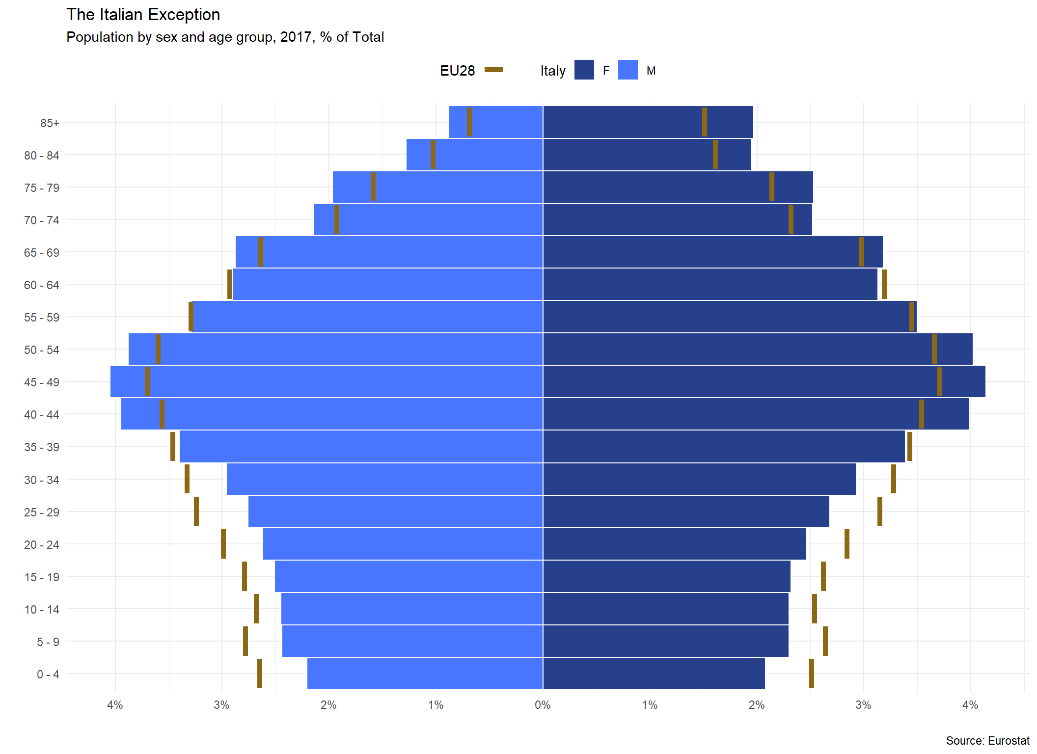
Inspiration from The Economist evaluating Italian aging population

Magazine Title: The Next Frontier

Article Title: Italy; Their Generation

Article Page: 35

Graph: The Italian Exception

Data Source: eurostat

Data Table Title: demo.pjan

Data Table Code: tps00001

Data Base Link:

I have read the data in locally, but there is also a great API wrapper eurostat package that can be used.

data_path <- "../../static/data/tt-eurostat-italy/"

age_cut <- seq(0,85,5)

fname <- dir_ls(data_path, regexp = ".tsv")

d <- read_tsv(fname, col_names = T)%>%
  select(contains("unit"), `2017`)%>%
  separate(.,col = "unit,age,sex,geo\\time", sep=",", into = c("unit", "age", "sex", "geo"))%>%
  filter(geo %in% c("IT", "EU28"))%>%
  filter(!age %in% c("TOTAL", "UNK"))%>%
  filter(!sex == "T")%>%
  filter(age != "Y_LT1" , age !="Y_OPEN")%>%
  mutate(age = as.numeric(str_replace_all(age, pattern="Y", "")), 
         value_2017 = as.numeric(str_replace_all(`2017`, pattern="[^0-9]", "")), 
         age_cut = cut(age, breaks = c(seq(0,85,5), Inf)))%>%
  select(-`2017`)
  

d_sub <- d%>%
  separate(age_cut, sep = ",", into = c("from", "to"), remove = F)%>%
  mutate_at(vars("from", "to"), str_replace_all, pattern = "[^0-9]","")%>%
  mutate(to = as.numeric(to)-1)%>%
  mutate(clean_lab = paste0(from, " - ", as.character(to)), 
         clean_lab = if_else(grepl(clean_lab, pattern = "NA")==T, "85+", clean_lab))%>%
  select(-c(unit, from, to))%>%
  group_by(geo)%>%
  mutate(tot_pop = sum(value_2017, na.rm = T))%>%
  group_by(sex, age_cut, clean_lab, add = T)%>%
  summarize(cohort_pop = sum(value_2017, na.rm = T), 
            pct_tot = cohort_pop/unique(tot_pop))%>%
  mutate(plot_value_pct = if_else(sex=="M", round((pct_tot*-1)*100,2), 
                                  round(pct_tot*100, 2)))%>%
  arrange(geo, age_cut)%>%
  ungroup()

Plot Italy population pyramid by age distribution and gender

eu28_bar <- filter(d_sub, geo == "EU28")%>%
  select(age_cut, sex, plot_value_pct)

ggplot(data = filter(d_sub, geo=="IT")%>%arrange(geo, age_cut), 
       aes(x = age_cut, y = plot_value_pct, fill = sex))+ 
  geom_bar(stat = "identity", width = 1, color = "white")+
  geom_errorbar(data=filter(d_sub, geo=="EU28")%>%arrange(geo, age_cut), 
                aes(ymax = plot_value_pct, ymin = plot_value_pct, 
                    color = "goldenrod4"), size = 1.85)+
  theme_minimal(base_family = "Roboto") + 
  scale_y_continuous(breaks = c(seq(-10, 10, 1)), 
                     labels = function(y) paste0(abs(y), "%"))+ 
  scale_x_discrete(labels = unique(d_sub$clean_lab)) + 
  scale_fill_manual(name = "Italy", values = c("royalblue4", "royalblue1")) + 
  scale_color_manual(name = "EU28", values = "goldenrod4", labels = NULL)+
  coord_flip() + 
  labs(x = "", 
       y = "", 
       title = "The Italian Exception", 
       subtitle = "Population by sex and age group, 2017, % of Total", 
       fill = "", 
       caption = "Source: Eurostat")+
  theme(legend.position = "top", 
        legend.direction = "horizontal")