More Housing Questions for 2021

Data sources & inspiration for visuals below:

1. U.S. Census & Appropriated Agencies - Population Estimates by Age Link to most recent survey

• Len Kiefer Freddie Mac - Population Growth and House Prices 2010 - 2018

2. U.S. Census - Geographic Mobility (All-Files, FileUsed (A-1))

• The Economist - The great slowdown
• Brookings Institute - William Frey

3. U.S. Average Primary Mortgage Market Rates (PMMS) - Freddie Mac PMMS

• Laurie Goodman - Urban Institute Housing Finance Policy Center (HFPC)
• Len Kiefer - Freddie Mac - Rate Spreads

4. National Association of Realtors (NAR) - Realtors Confidence Index (c)

• FRBNY - Liberty Street Economics (blog)

NOTE The majority of these data are dated as we are looking at longer term trends. Much of the data was captured, tabulated and reported prior to full impact of Covid-19 and restriction policies being put in place. Therefore, the data may be subject to substantial revisions and/or changes within subsequent releases.

if(!require(pacman)){
  install.packages("pacman")
  require(pacman)
}

p_load(tidyquant, tidyverse, lubridate, purrr,
       tools, fs, scales, readr, readxl, 
       ggdark, colorspace, crayon)

# Set filepath for where local data is stored. 
# This includes the Age demographic data and proportion of first time homebuyers

data_path <- "../../static/data/mtg_2021/"


# Set colors that will be used for plots near the end

col_point_line_charts <- colorspace::sequential_hcl(palette = "Dark Mint", n = 1)[1]
fill_fthb <- colorspace::sequential_hcl(palette = "Dark Mint", n = 3)[c(1,2)]

Questions: positive view v. negative view with graphs

1. What does the composition of the age demographics of the population mean for housing going forward?

+ Millennial’s, particularly those children of the baby boom era continue to suggest ongoing high demand for new home purchases. Those aged 27 as of 2018 (i.e. presently 29) are 4.81 million individuals who will continue to drive demand as they form households and look to purchase homes (if they have not already). As of 2019, the median age of first-time home buyers (FTHB) is estimated to be 33 by the National Association of Realtors (NAR).

- Despite this demographic tailwind, first-time home buyers (FTHB) continue to remain lower than expected relative to demand (see more below)

- The pandemic and higher costs to build is likely to continue to put negative pressure on prospective entrants to the purchase market.

# p_fthb_pop_lab <- filter(d_pop_sub, age == 27 | age == 32)%>%
#   mutate(lab_txt = ifelse(age == 27, "Largest population by age", 
#                           "Median age - first time homebuyer"))

p_pop_fthb <- d_pop_sub%>%
  ggplot(.)+
  geom_bar(aes(x = age, y = value_millions, fill = generation_name), 
           stat = "identity",alpha = 0.7, size=0.1)+
  scale_fill_discrete_sequential("Dark Mint", 
                                 guide = guide_legend(
                                   direction = "horizontal",
                                   label.position = "top", 
                                   title = "", 
                                   reverse = T, 
                                   keywidth = unit(1.5, "cm")))+
  scale_color_manual(values = c("black"), guide = FALSE)+
  scale_x_continuous(labels = seq(18,85,3), 
                     breaks = seq(18,85,3))+
  scale_y_continuous(breaks = seq(0,5,.5), 
                     labels = function(x) paste0(x, "M"))+
  labs(title = "U.S. population by age as of 2018",
       subtitle = NULL, 
       x = "Age",
       y= "Population (M)",
       caption = NULL)+
  ggdark::dark_theme_minimal()+
  theme(legend.position = "top")


p_pop_fthb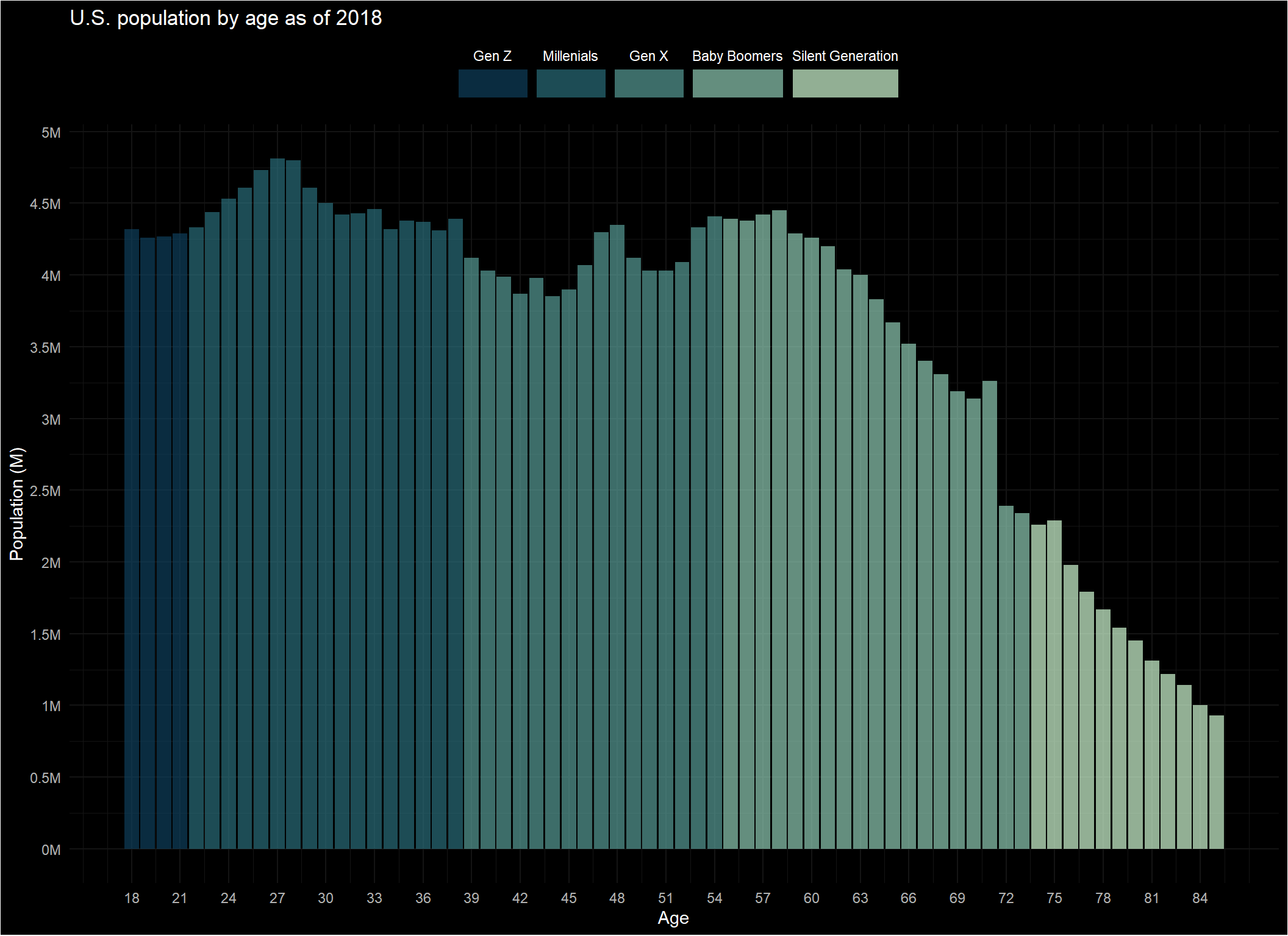

2. What does the secular trend in declining mobility within the U.S. mean for the future of owner-occupied housing?

+ Mobility and movement creates the opporutnity for more transactions of new and existing home sales. Demographic trends may provide a positive impact to this trend as: 1. Younger generations coming of age (28-35 year old’s) consider moves from cities to suburbs for lifestyle reasons (better school district, more affordable cost/sq. ft. for growing families, etc.) or reduction in usage of amenities (under pandemic conditions or otherwise) 2. Likewise, older generations (baby-boomers) may downsize as children leave the home, maintenance and accessibility are not accommodating to their age or retirement enables a desired move (e.g. to warmer climates).

- Increased remote work and digitally enabled careers further reduces the proportion of the population needing to relocate for work

- Low inventory in homes available for sale make the prospects or interest of moving less desirable when purchaser’s feel they would be over-stretched financially and hold out until more listings are available.

In the event mortgage rates begin to rise, those with existing mortgages have a further disincentive to move if they have capitalized on historic lows in mortgage rates.

# Get label for most recent reporting period
mobility_lab_curr <- d_mobility_pct_sub%>%
  slice(which.max(xlab_end_date))
  
p_mobility <- d_mobility_pct_sub%>%
  ggplot(aes(x = xlab_end_date, y = tot_move))+
  geom_line(size = 1.33, color = "white")+
  geom_point(data = mobility_lab_curr, aes(x = xlab_end_date, y = tot_move), 
             size = 4.25, alpha = 0.85,
             fill = col_point_line_charts, color = col_point_line_charts)+
  geom_text(data = mobility_lab_curr, 
             aes(x = xlab_end_date, y = tot_move, 
                 label = paste0(tot_move,"%")), 
             color = "white", vjust = -1, hjust = -.025, fontface = "bold")+
  scale_y_continuous(limits = c(0,25), breaks = seq(0,25, 2), 
                     labels = function(y) paste0(y, "%"))+
  scale_x_date(date_breaks = "5 years", date_labels = "%Y")+
  labs(title = "Mobility in the US", 
       subtitle = "Technologically mobile, depressing real mobility", 
       x= "End of survey year (Mar-YY)", 
       y= "% moved in last year", 
       caption = "U.S. Census Bureau \n **Note survey ends in March (pre-Covid for 2020)")+
  theme_minimal()+
  dark_theme_minimal()


p_mobility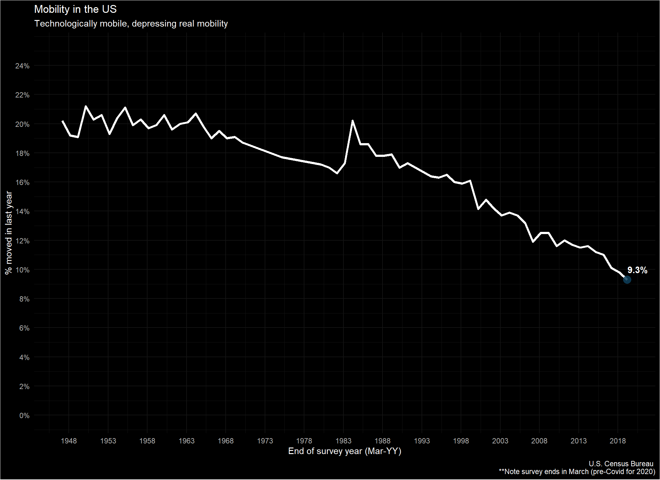

3. How many people will be priced out if mortgage finance rates begin to elevate?

The post Great Recession period of low interest rates has been beneficial to housing, particularly existing mortgage holders eligible for refinancing. However, many have not been able to capitalize on the more affordable rates due to economic factors (unemployment during the Great Recession or Covid-19). In recent years, increased home prices and soaring rents likely contributed in diminishing the benefits of low rates contribution to mortgage affordability.

rate_lab_curr <- d_rate_natl%>%
  select(dt_full = date, mtg30_yr_frm)%>%
  slice(which.max(dt_full))

p_rate <- select(d_rate_natl, dt_full = date, mtg30_yr_frm)%>%
  mutate(dt_yr = year(dt_full)%>%as.numeric(), 
         mo_num = month(dt_full)%>% as.numeric(), 
         mo_abb = month.abb[mo_num])%>%
  filter(dt_yr > 1999)%>%
  ggplot(.)+
  geom_line(aes(x = dt_full, y = mtg30_yr_frm), size = 1.33)+
  geom_point(data = rate_lab_curr, aes(x = dt_full, y = mtg30_yr_frm), 
             size = 4.25, alpha = 0.85,
             fill = col_point_line_charts, 
             color = col_point_line_charts)+
  geom_text(data = rate_lab_curr, 
            aes(x = dt_full, y = mtg30_yr_frm, 
                label = paste0(mtg30_yr_frm,"%")), 
            color = "white", vjust = 1.75, fontface = "bold")+
  scale_x_date(date_breaks = "9 months", date_labels = "%b-%Y")+
  scale_y_continuous(breaks = seq(0,9,1.25), labels = function(y) paste0(y,"%"), 
                     limits = c(0,9))+
  labs(title = "Longterm secular trend in low-interest rates", 
       subtitle = "30-Year fixed rate mortgage", 
       x = NULL, 
       y = NULL,
       caption = "Freddie Mac, PMMS")+
  dark_theme_minimal()+
  theme(axis.text.x = element_text(angle = 45))

p_rate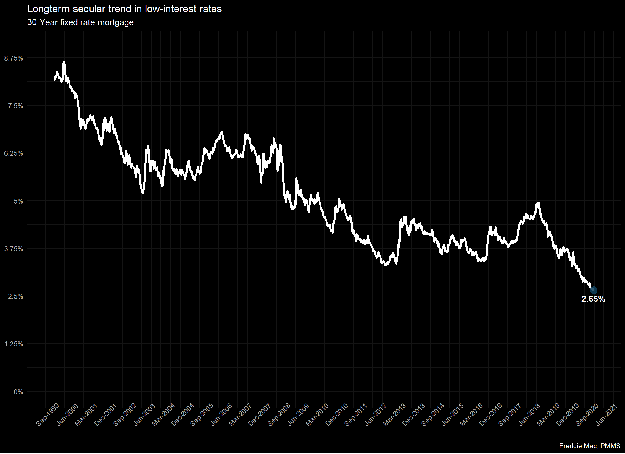

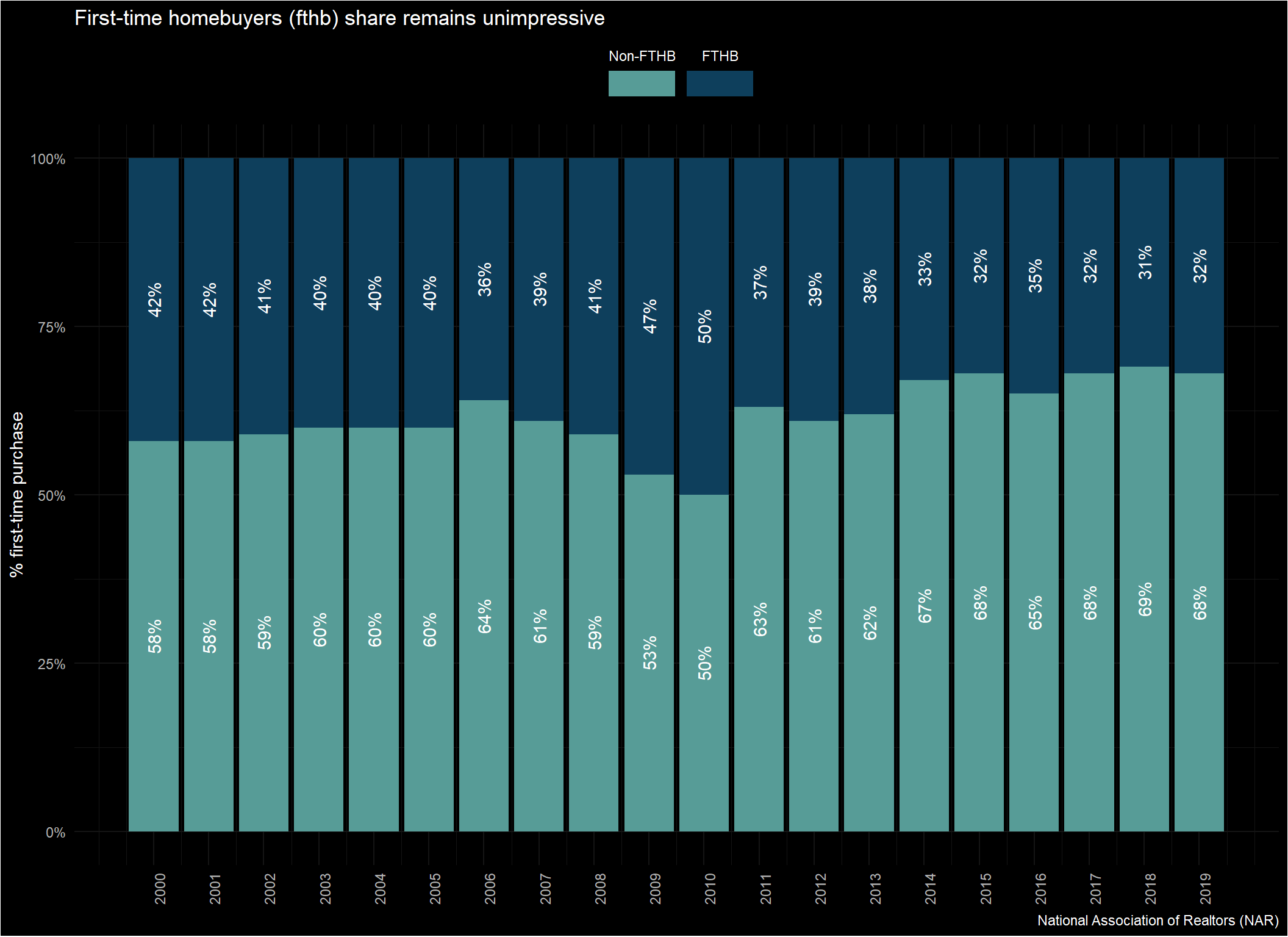
4. Will the proportion of first-time home buyers (FTHB) increase in-line with demographic trends?

+ Given the positive demographic trends and lower rate environment – a future increase in available inventory of homes for sale could quickly lead to strong demand for new first-time home buyers.

- As expected, the rate shrunk after the Great Recession, yet the sustained lower proportion of first-time home buyers has persisted longer than expected.

- Economic uncertainty under Covid-19 has the potential to further stem growth and home-purchases by new entrants.

p_fthb <- d_fthb_pct%>%
  ggplot()+
  geom_bar(stat = "identity", aes(x = dt_yr, y = value, group = name, fill = name), 
           position = "stack")+
  geom_text(aes(x = dt_yr, y = value, group = name, 
                label = paste0(round(value*100,0),"%")), 
            position = position_stack(vjust = .5), 
            angle = 90, color = "white")+
  scale_y_continuous(labels = percent)+
  scale_x_continuous(breaks = seq(2000,2019,1))+
  scale_fill_manual(values = fill_fthb, 
                    guide = guide_legend(
                                     direction = "horizontal",
                                     label.position = "top", 
                                     title = "", 
                                     reverse = T, 
                                     keywidth = unit(1.5, "cm")))+
  labs(title = "First-time homebuyers (fthb) share remains unimpressive", 
       x = NULL, 
       y = "% first-time purchase",
       caption = "National Association of Realtors (NAR)")+
  dark_theme_minimal()+
  theme(legend.position = "top", 
        axis.text.x = element_text(angle = 90))
  
p_fthb