Seattle Comprehensive Plan - Part III - Progress

Methodology Notes

Similar to previous posts, I will not detail out the specific methodologies utilized to generate these data. However, further high-level reading can be done at the following sites:

1. Zillow home sales
2. Zillow Home Value Index (ZHVI) - Summary Method, Zillow HVI - Deep Dive
3. Freddie Mac PMMS

In addition, there are a number of “gotchas” when comparing this many data sources, geographies and time intervals. I do not account for a number of these in this particular post given our interest in high-level trending.

Inventory of Homes for Sale in Months

About the measure: This is a common supply side measure used to evaluate the temperature of a real estate market for existing or new home purchasers and sellers. The measure output can be understood as: given the current number of home sales, how many months would it take to sell all of the properties listed (i.e. how much housing stock is available to choose from for prospective buyers).

Impact of measure: Month’s of inventory can be distilled down into two specific output categories based on whether there is a glut of supply (excess supply, relative to demand) or a dearth (scarcity of supply, relative to demand). The measure is generally interpreted within the context of it’s relationship to: (i) existing and future home prices; (ii) length of time a listing is available on the market and (iii) whether the actual sales price is below, equal to or above the listed price.

0. Equilibrium (supply=demand): The general industry rule of thumb based on historic data indicate that a measure of 4.5 - 5.5 months is indicative of a housing market in equilibrium. Said simply, when the inventory is at that level – we do not expect to see upward or downward pressure on home prices, relative to their long-term fundamentals.

1. Sellers Market (supply < demand): If the month of inventory is below our equilibrium value, we call this a sellers market. The market is termed as such because the lack of available homes for sale puts upward pressure on home prices indicating the higher likelihood that sellers will receive their actual or above listing price.

2. Buyers Market (supply > demand): Conversely, when there are more available homes than buyers (e.g. first time home buyers), those seeking to buy are benefited because they have more options available and thus more bargaining power.

d_supply_compare%>%
  select(dt_full, contains("inventory"))%>%
  rename(`Seattle Monthly Inventory` = mo_inventory_z, 
         `National Monthly Inventory` = mo_inventory_natl)%>%
  gather(variable, value, -"dt_full")%>%
  ggplot()+
  geom_bar(stat = "identity", aes(x = dt_full, y = value, group = variable, fill = variable), 
           position = "dodge")+
  geom_hline(yintercept = 5.5, linetype = 2, color = "darkred")+
  scale_fill_viridis_d("")+
  scale_x_date(date_breaks = "6 months", date_labels = "%Y-%B")+
  theme_minimal()+
  labs(title = "Comparing National v. Seattle by Month's Supply of Housing", 
       subtitle = NULL, 
       x = NULL, 
       y = "# of Months", 
       caption = "Zillow, U.S. Census, Housing and Urban Development")+
  theme(legend.position = "top", 
        axis.text.x = element_text(angle = 90))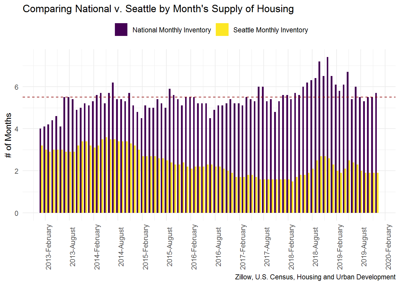

Average Monthly Mortgage Payment

About the measure: Average monthly mortgage payment is utilized for understanding what the estimated monthly housing payment expense would be for a household by utilizing: (i) current average rates (national) and (ii) the current median home price value (by locale). The two largest components of mortgage payments are principal and interest (P+I). There are additional monthly recurring costs such as insurance and taxes, which we will not include here.

Impact of measure: Each of the two inputs has the potential to increase or decrease the average monthly mortgage. Mortgage rates are set by the lending institution based on a multitude of factors and median home prices are driven by supply and demand components. Given the proportion of monthly expense usually associated with shelter (either monthly mortgage or rent), this metric provides a good read on how expensive housing is within a geography. For now we will just evaluate the raw figures, but in future posts we may further unpack some of these concepts. Specifically, what monthly housing expense means relative to wage and income for an area.

Note on assumptions: For our payment calculation, there are a few sets of assumptions beyond the earlier mention that this is not an “all-in” payment amount. In general, the output from our calculations can be presumed to be lower (or more conservative), than the actual monthly mortgage obligation. 1. We assume a 10% upfront down payment. Despite the anecdote that you should have 20%, that is not and has not been a reality for quite some time. According to the National Association of Realtors (NAR) most recent survy estimated that 76% of new home buyers put down less than 20%, while 56% of existing home buyers put down less than 20. Zillow has produced similar survey figures as well.

d_mtg_compare%>%
  select(dt_full, contains("avg_pmt"))%>%
  rename(`Avg. Pmt Seattle` = avg_pmt_local, `Avg. Pmt National` = avg_pmt_natl)%>%
  gather(variable, value, -"dt_full")%>%
  mutate(dt_yr = as.character(year(dt_full)))%>%
  ggplot()+
  geom_bar(stat = "identity", aes(x = dt_full, y = value, fill = variable, group = variable), 
           position = "dodge")+
  scale_y_continuous(labels = dollar)+
  scale_x_date(date_breaks = "9 months")+
  scale_fill_viridis_d("")+
  theme_minimal()+
  theme(legend.position = "top", 
        axis.text.x = element_text(angle = 90))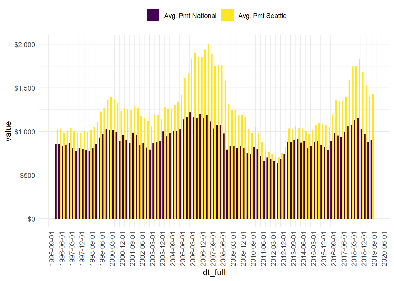

Median Gross Rent (tract aggregated to county and city boundaries)

About the measure: The Census conducts frequent surveys in order to evaluate households and individuals on an interim basis between decennial Census surveys. For this post, we’ll evaluate gross rents, which combines contract rent (monthly rental expense) and average utilities.

Impact of measure: The previous measures are specific to affordability with respect to existing or prospective homeowners, while median gross rent provides additional details into the monthly housing burden for households renting.

# Distribution of Gross Rent by Tracts within King county
ggplot(d_kc_rent, aes(estimate))+
  geom_histogram(fill = "navy", bins = 60, color = "white")+
  scale_x_continuous(labels = scales::dollar, breaks = seq(0, 3750,375))+
  facet_wrap(~dt_yr, ncol = 1)+
  theme_minimal()+
  geom_vline(aes(xintercept = median_val, group = dt_yr), lty = "dashed", size = 1, 
             color = "darkgreen")+
  geom_text(aes(label = paste0("Median Value: $", prettyNum(median_val, big.mark = ",")), 
            x = median_val+1000, y = 20))+
  labs(title = "King County gross rent by tract", 
       subtitle = "Comparing 2014 to 2018",
       x = "Monthly Gross Rent ($s)",
       y = "Tract Cnt",
       caption = "ACS-5yr Survey, U.S. Census")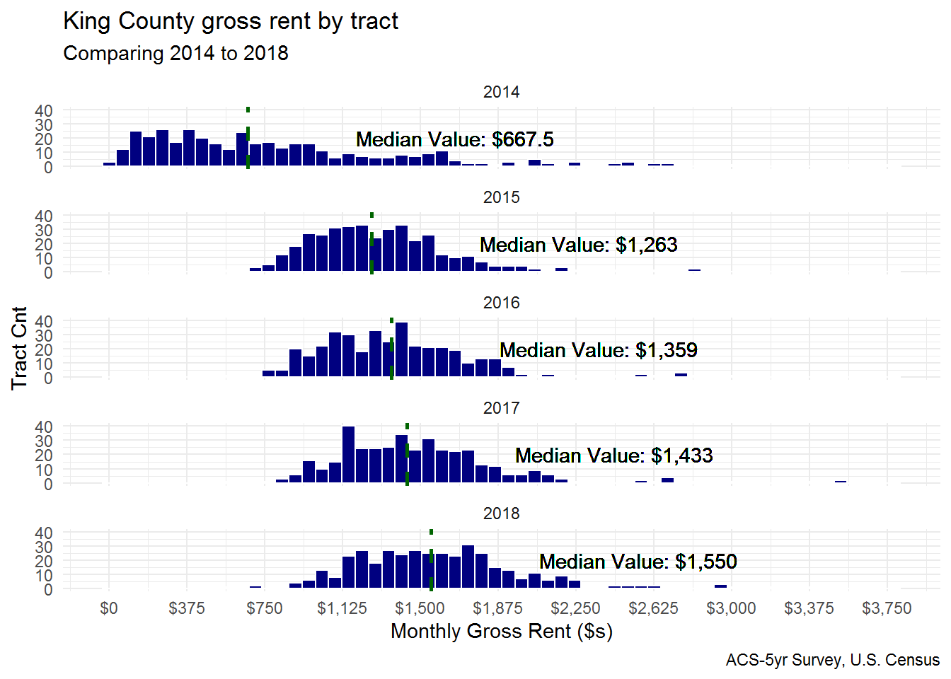

# Distribution of Gross Rent by Tracts within Seattle

ggplot(d_sea_rent, aes(estimate))+
  geom_histogram(fill = "navy", bins = 60, color = "white")+
  scale_x_continuous(labels = scales::dollar, breaks = seq(0, 3750,375))+
  facet_wrap(~dt_yr, ncol = 1)+
  theme_minimal()+
  geom_vline(aes(xintercept = median_val, group = dt_yr), lty = "dashed", size = 1, 
             color = "darkgreen")+
  geom_text(aes(label = paste0("Median Value: $", prettyNum(median_val, big.mark = ",")), 
                x = median_val+1000, y = 10))+
  labs(title = "Seattle gross rent by tract", 
       subtitle = "Comparing 2014 to 2018",
       x = "Monthly Gross Rent ($s)",
       y = "Tract Cnt",
       caption = "ACS-5yr Survey, U.S. Census")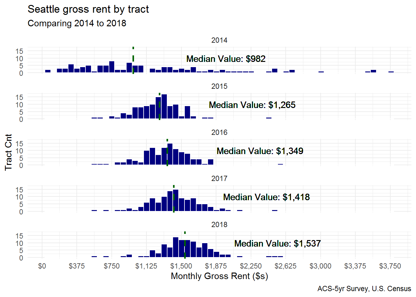

A map for fun…

# Map Tract Data For Seattle

# Create Clean Theme For Map
theme_map_sq <- function(...){
  theme_minimal()+
    theme(
      text = element_text(family = "Arial Narrow", color = "#22211d"),
      axis.line = element_blank(),
      axis.text.x = element_blank(),
      axis.text.y = element_blank(),
      axis.ticks = element_blank(),
      axis.title.x = element_blank(),
      axis.title.y = element_blank(),
      # panel.grid.minor = element_line(color = "#ebebe5", size = 0.2),
      panel.grid.major = element_line(color = "#ebebe5", size = 0.2),
      panel.grid.minor = element_blank(),
      plot.background = element_rect(fill = "#f5f5f2", color = NA), 
      panel.background = element_rect(fill = "#f5f5f2", color = NA), 
      legend.background = element_rect(fill = "#f5f5f2", color = NA),
      panel.border = element_blank(),
      legend.title.align = 0.5, 
      legend.position = c(0.5, -0.07),
      legend.box.background = element_rect(fill = NA, color = NA),
      legend.key = element_rect(color = "transparent", fill = "white"),
      ...
    )
}

# Set Break Length for Clean Categories
brk_length <- 7

# Create Clean Labels Based on Breaks and Build Map Faceted by ACS Survey Year
d_sea_rent%>%
  mutate(brk_value = cut(estimate, pretty(d_sea_rent$estimate, n = brk_length),
                         dig.lab = 4))%>%
  separate(brk_value, sep=",", into = c("from", "to"), remove = F)%>%
  mutate_at(c("from", "to"), 
            ~str_replace_all(., pattern = "[^[:alnum:]]", "")%>%as.numeric())%>%
  mutate_at(c("from","to"), ~case_when(
    . > 999 ~ paste0(as.character(./1000), "K"), 
    . < 1000 ~ as.character(.)))%>%
  unite("brk_val_lab", from,to, sep = " to ")%>%
  mutate(brk_val_lab = factor(brk_val_lab, 
                              levels = c("0 to 500", "500 to 1K", 
                                         "1K to 1.5K","1.5K to 2K", 
                                         "2K to 2.5K", "2.5K to 3K", 
                                         "3K to 3.5K","3.5K to 4K")))%>%
  ggplot()+
  geom_sf(aes(fill = brk_val_lab), color = "white")+
  theme_map_sq()+
  theme(legend.position = "bottom")+
  scale_fill_manual(
    values = viridis(8, alpha = 0.9), 
    na.value = "grey60",
    name = "Gross Rent ($)",
    guide = guide_legend(
      direction = "horizontal",
      keywidth = unit(1.75, "cm"),
      nrow = 1, 
      byrow = T,
      title.position = "top", 
      label.position = "bottom", 
      title.hjust = 0.5))+
  facet_wrap(~dt_yr, nrow = 1)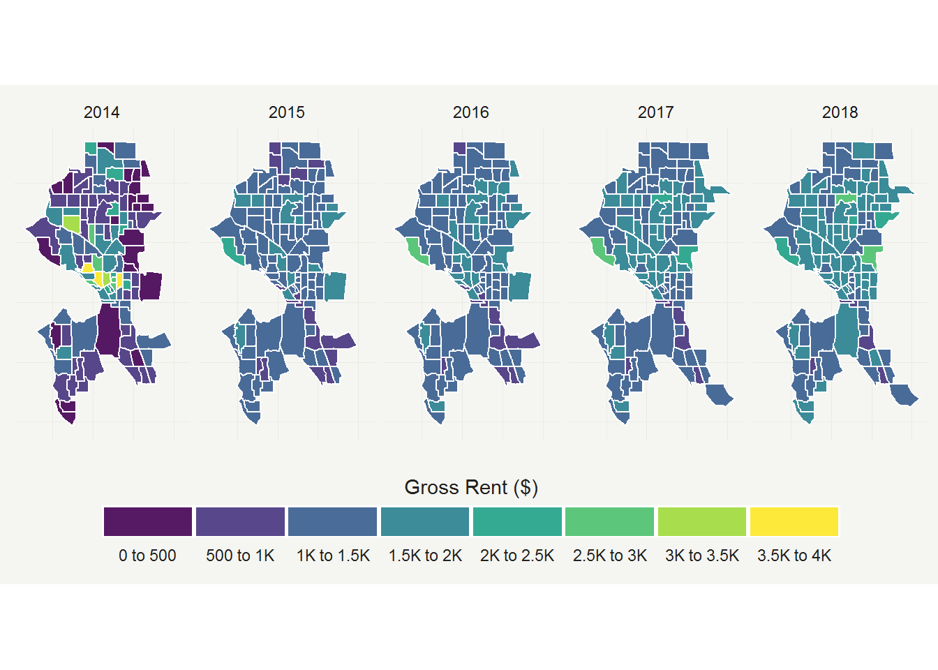

Observations and Conclusions

• For the city of Seattle and surrounding areas inventory of homes for sale remains low. Assuming demand remains consistent, we would continue to see minor upward pressure on home prices though there could be leveling off after a long period of it being a “sellers” market. Based on the plot, it appears we would expect to see nationwide home price appreciation begin to move toward the long-term range – moderating from sizeable increases
• Monthly mortgage payments are expensive relative to what is paid nationally. Seattle (and the rest of the nation) has largely benefited from historic lows in interest rates. Despite this trend in interest rates, home sale values still make Seattle an expensive city
• Rents have continued to increase over time - particularly from 2014 - 2015, where King County saw median rents nearly double. This trend moderated over time, particularly within Seattle – though these monthly costs continued to expanded outward spreading the cost more broadly to periphery tracts/neighborhoods.