A Growth Strategy Evolution
Last week the Seattle Planning Commission released an interim white paper titled Evolving Seattle’s Growth Strategy – foreshadowing their updates to the Commission’s revised Comprehensive Plan due in 2023.
The white paper, builds off the foundation Seattle 2035 - Growth and Equity report (May, 2016) and the Commissions most recent Neighborhoods for All reports.
A Quick Background
The Planning Commission
The Seattle Planning Commission is an independent, 16-member advisory body appointed by the Mayor, City Council, and the Commission itself. The members of the Commission are volunteers who bring a wide array of expertise and a diversity of perspectives to these roles.
The Legal Directive(s)
A RESOLUTION affirming the City’s race and social justice work and directing City Departments to use available tools to assist in the elimination of racial and social disparities across key indicators of success, including health, education, criminal justice, the environment, employment and the economy; and to promote equity within the City workplace and in the delivery of City services.
2014 - Executive Order 2014-02 >This Executive Order affirms the City of Seattle’s commitment to the Race and Social Justice Initiative (RSJI), and expand RSJI’s work to include measurable outcomes, greater accountability, and community wide efforts to achieve racial equity in our community.
2015 - Adoption of Resolution 31577 >A RESOLUTION confirming that the City of Seattle’s core value of race and social equity is one of the foundations on which the Comprehensive Plan is built
The city of Seattle realized early on the potential dark sides of urban growth and attempted to provide thoughtful forward planning through a set of strategic and policy remedies that could potentially stem the strain on current and future residents.Though there are many contributing factors to the cities rapid growth (for instance the beautiful natural amenities, temperate climate, etc.), the reality likely resides more so within the expansion of the technology sector and gainful employment. Amazon company growth and signaling in 2017 of targeting 100,000 new hires, coupled with unaffordable housing conditions in nearby San Francisco likely increased in-migration to the city of Seattle.
Net Migration for King County
Using the wonderful R package tidycensus, we’ll quickly take a look at annual migration growth for King County, WA (of which Seattle is a part of) with a few lines of code. In addition, we’ll quickly compare the population distributions by race between 2010 and 2018. Note: A U.S. Census api key is required to use tidycensus.
The majority of the data is self-contained within the tidycensus::get_estimates wrapper calling the API, but we’ll add a few extra steps simply for describing the categories pulled down. As usual, we’ll be utilizing tidyverse (stringr, ggplot2, dplyr, rvest) and the scales package for consuming and plotting the data below.
Retrieving the data from Census API
- First we’ll create reference tibbles to join to our data set on code id
- Then source the data from U.S. Census
- Net migration population component (2010 through 2018)
- Proportion of population by race (2018 v. 2010)
- Join reference tables to Census data on codes
# Per tidycensus documention, you may need to load API
# census_api_key("YOUR API KEY GOES HERE")

# Reference Tables:
#1. Migration Estimates Reference
kc_yr <- tibble(ts_per = seq(1,8,1),
                ts_yr_from = seq(2010, 2017, 1),
                ts_yr_to = seq(2011, 2018, 1),
                ts_lab = paste("From", ts_yr_from, "to", ts_yr_to))

#2. Racial Demographic Reference table (using rvest package to scrape table)

# Get site url
# Once on site, right-click - > inspect to find the html code, then right click to copy
# the xpath
race_url <- "https://www.census.gov/data/developers/data-sets/popest-popproj/popest/popest-vars/2018.html"
race_xpath <- "//*[@id='detailContent']/div/div/div[8]/div[2]/div[1]/div"

kc_race_ref <- read_html(race_url)%>%
  html_nodes(xpath = race_xpath)%>%
  html_nodes("p")%>%
  html_text()%>%
  tibble("cd_in"=.)%>%
  separate(cd_in, sep="=", into = c("race_cd", "race_desc"))%>%
  na.omit()%>%
  mutate(race_cd = as.numeric(race_cd))


# Source Data **NOTE** product variable setting

# NET MIGRATION for KING COUNTY, time_series gives us data from 2010 to current
kc_component <- get_estimates(geography = "county", state = "53",
                              county = "033", time_series = T, product = "components")%>%
  filter(variable == "NETMIG")%>%
  left_join(., kc_yr, by = c("PERIOD"="ts_per"))

# Population by Race (raw figures, converted into proporitions)
# Not product variable and breakdown variable

kc_race <- bind_rows(
  get_estimates(geography = "county", state = "53",
                         county = "033", year = 2018, product = "characteristics",
                         breakdown = "RACE")%>%
    mutate(rep_yr = 2018),
  get_estimates(geography = "county", state = "53", county = "033",
                year = 2015, product = "characteristics", breakdown = "RACE")%>%
    mutate(rep_yr = 2010)
)%>%
  left_join(., kc_race_ref, by = c("RACE"="race_cd"))%>%
  filter(RACE != 0)%>%
  mutate(dt_yr_f = as_factor(rep_yr))%>%
  group_by(dt_yr_f)%>%
  mutate(prop_race = value/sum(value, na.rm = T))%>%
  ungroup()
Plot data
We can quickly see that King County (of which Seattle is a part of), has a couple of outstanding trends – a highly homogeneous population (predominately White) and large net in-migration growth (hence the city planning).
# Net Migration

p_netmig <- kc_component%>%
  ggplot()+
  geom_bar(stat = "identity", aes(x = reorder(ts_lab, -PERIOD), y = value), fill = "navy")+
  coord_flip()+
  scale_y_continuous(labels = scales::comma)+
  theme_minimal()+
  labs(title = "King County Net Migration",
       subtitle = "From 2010 to 2018",
       x = NULL,
       y = "Persons")

# Race proportion distribution. Comparing 2010 to 2018

p_kc_race <- kc_race%>%
  ggplot()+
  geom_bar(stat = "identity", aes(x = reorder(race_desc, prop_race), y = prop_race, group = dt_yr_f, fill = dt_yr_f),
           position = "dodge")+
  coord_flip()+
  scale_x_discrete(labels = function(x) str_wrap(x, 35))+
  scale_y_continuous(labels = scales::percent)+
  scale_fill_manual("",values = c("navy", "darkred"))+
  theme_minimal()+
  theme(legend.position = "top")+
  labs(title = "King County Population by Race (Proportion)",
       subtitle = "Comparing 2018 to 2010 Estimates",
       x = NULL,
       y = "Pop % Est.")

p_netmig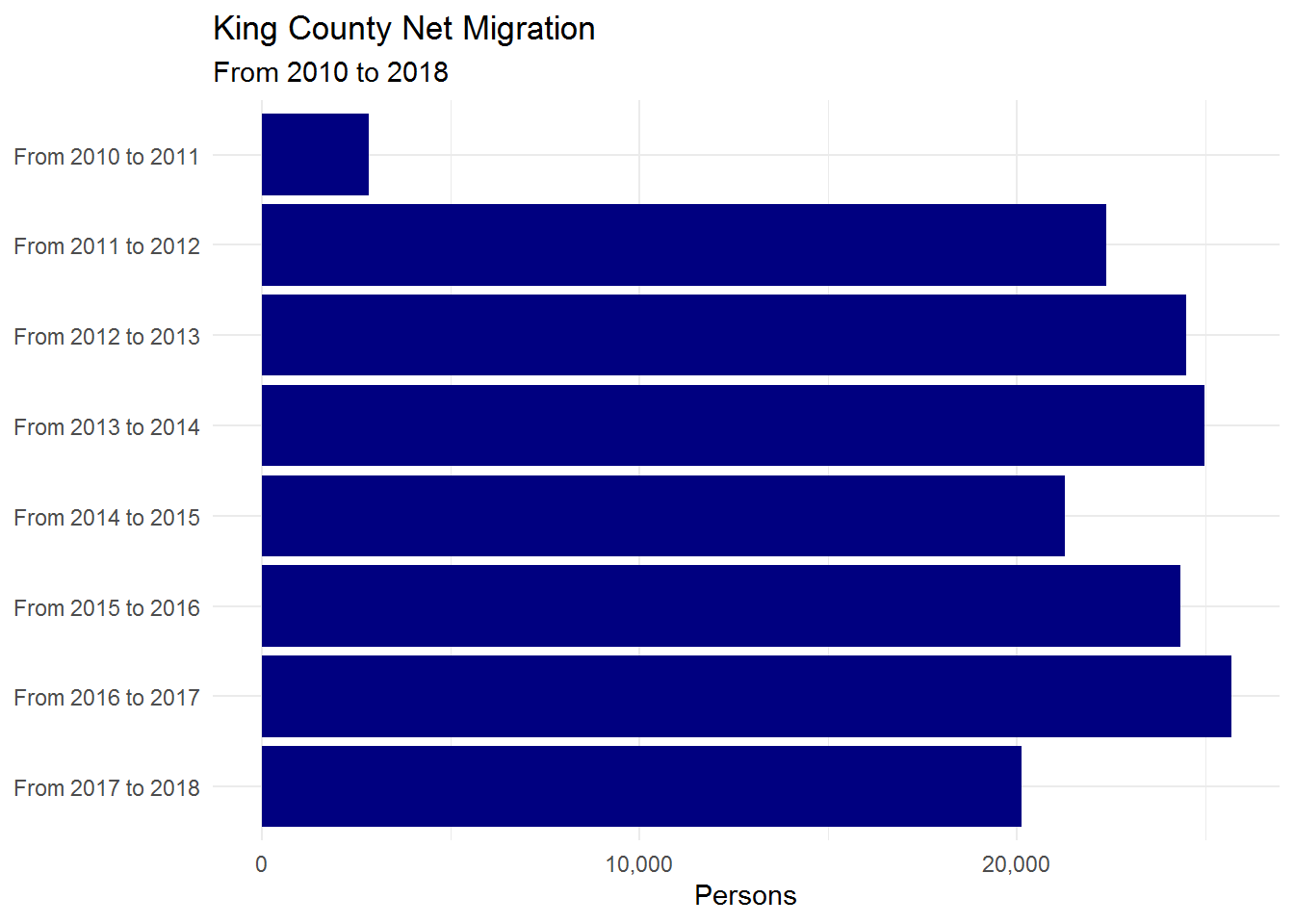
p_kc_race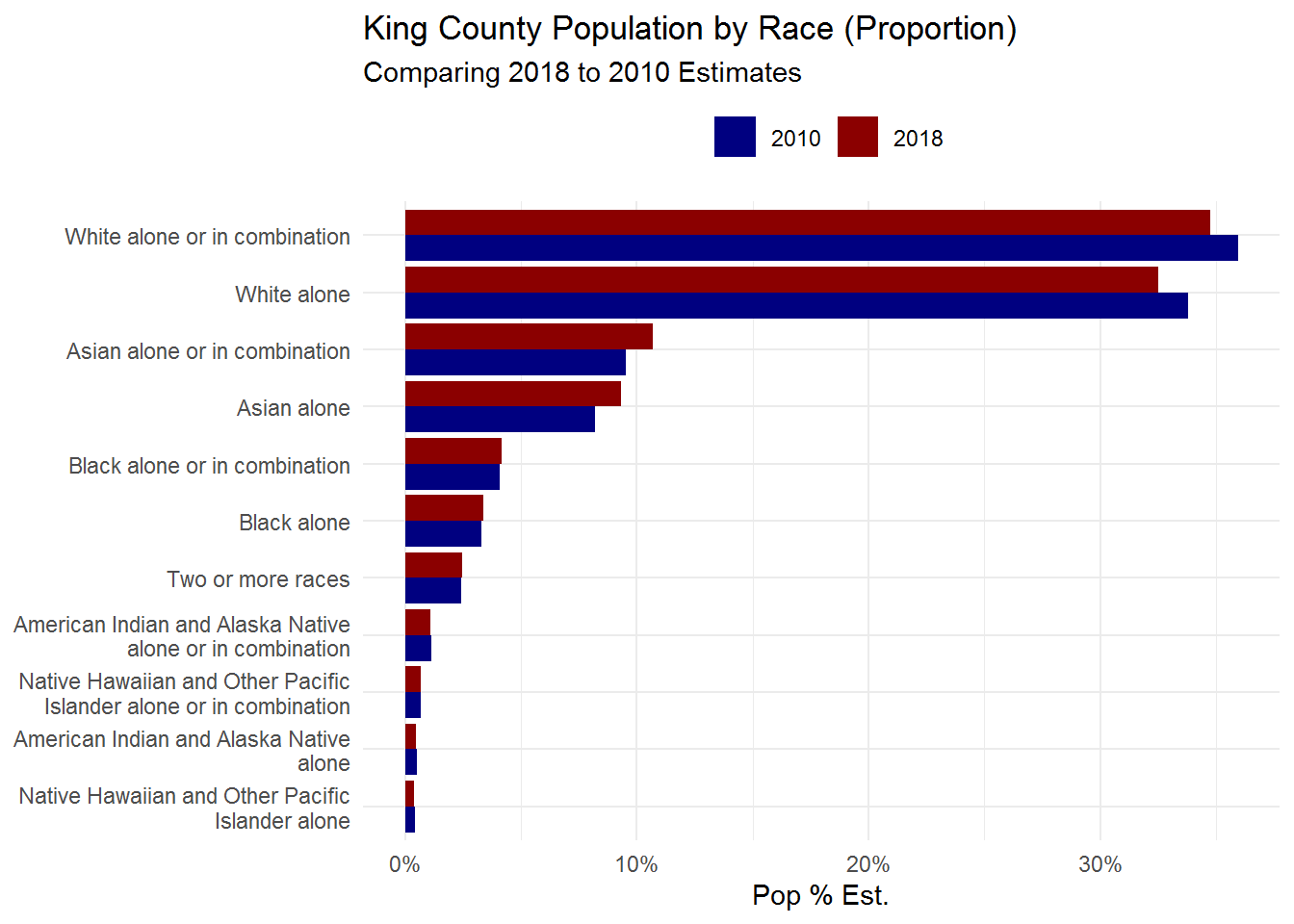
Conclusion and Next Steps
We see there is clearly a looming problem, in a future post we’ll use our combination of tidycensus along with sf (simple features) and leaflet package to recreate some of the maps contained within the updates to track progress of the 2035 plan to date based on the most recent report…