Sizing the U.S. Residential Mortgage Market (Part I)

Sizing U.S. Residential Mortgage Markets

The U.S. residential mortgage market is one of the most unique in the world given the secondary market financing structure enabled by private market participants and government programs. It is followed not only by your average consumer looking for shelter, but also by:

• politicians at every jurisdictional level
• advocates and academics
• investors and analysts and
• regulators

Just to name a few….

A quick rundown on terminology

There thousands of metrics and measure monitored to evaluate opportunities and lurking risks in housing. This first post will simply cover some of the key aggregate national market measures. First, a few key terms and definitions:

1. Residential: Generally (and for this post), we mean 1 - 4 unit single family residences / duplexes and town homes (some measures include manufactured housing as well).
2. Mortgage: Financing instrument with accompanying deed indicating the amount owed (debt). This will exclude rentals and leases
3. Origination: The face value of money owed on the mortgage note when closing
4. Debt: Remaining balance owed by an individual to a financial institution
5. Equity: Value owned by an indivdaidual or non-profit through principal payments on mortgage and/or accrued through appreciation in the house and the land it is affixed.

Measure types:

1. Stock: The total level of the unit in question
2. Flow: The inflow or outflow of the unit in question modifying the total stock of unit

These are very high-level summary of terms – there are a myriad of sources that unwind the nuances and criteria.

So just how big of a market is it?

For this post, we’ll cover a standard set of metrics. Each metric varies slightly and helps analysts or individuals understand the magnitude of the U.S. residential housing market in terms of $’s.

1. Annual Originations (Flow | $’s): The number of new mortgages (purchase loans and re-finances). (Flow Metric)

2. Mortgage Share as Percent of Originations (Flow | %): The percent of originations in $’s as a percent of total originations, segmented by the end investor who owns rights to the underlying asset in the event of non-repayment.

3. Total Homeowners Equity (Stock | $): The amount of equity/value available to individuals who own their home partially or outright

Note about the code

The work horse for this analysis (and most analysis) is tidyverse, tidyquant and lubridate. Since we are working with time-series data, tidyquant is of particular use given it’s ability to call the St. Louis maintained Federal Reserve Economic Data (FRED) datasets quickly into your environment.

Data is sourced primarily from government sources, though some data is tracked and published by commercial entities.

Data Analysis

fname <- "../../static/data/1_mtg_mkt_share/20190102_Combined_Mtg_Size_File.xlsx"

ref_sheet_nm <- excel_sheets(fname)

d_orig <- read_excel(fname, sheet = ref_sheet_nm[1])

d_orig_avg <- d_orig%>%
  mutate(dt_full = ymd(dt_full))%>%
  group_by(dt_full, loan_purpose)%>%
  summarize(avg_vol_bil = mean(value, na.rm = T))%>%
  ungroup()%>%
  mutate(cln_lab = paste0("$", prettyNum(round(avg_vol_bil, 0),big.mark = ",")))

est_avg19 <- filter(d_orig_avg, year(dt_full) == 2019)%>%
  group_by(loan_purpose)%>%
  summarize(tot19_bil = sum(avg_vol_bil, na.rm = T))%>%
  spread(loan_purpose, tot19_bil)%>%
  mutate(Title = "Total Est. Origination ($B)", 
         `Est. Total` = Purchase + Refinance)%>%
  select(Title, Purchase, Refinance, `Est. Total`)%>%
  mutate_if(is.numeric, ~.x%>%round(.,0)%>%prettyNum(., big.mark = ","))

p1_orig <- d_orig_avg%>%
  ggplot()+
  geom_bar(stat = "identity", aes(x = dt_full, y = avg_vol_bil, fill = loan_purpose), 
           position = "stack")+
  scale_fill_viridis_d("")+
  scale_x_date(date_labels = "%Y-%m", date_breaks = "3 months")+
  scale_y_continuous(label = dollar)+
  labs(title = "Avg. estimated quarterly originations", 
       subtitle = "By loan purpose", 
       x = NULL, 
       y = "$B", 
       caption = "Source: MBA, Fannie Mae, Freddie Mac")+
  theme_minimal()+
  theme(legend.position = "top")
  
p1_orig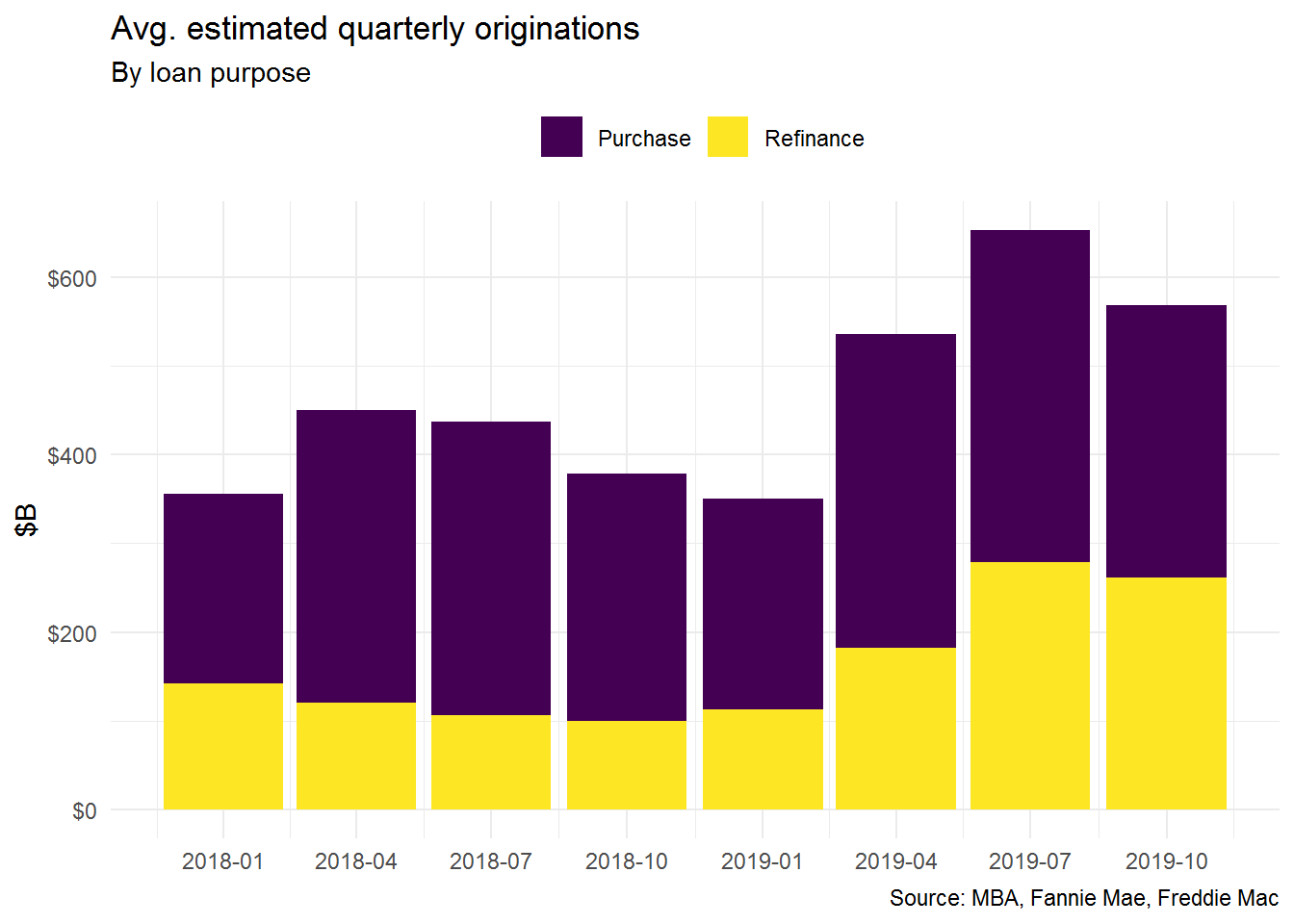

est_avg19%>%
  kable()

Investor share as percent of origination volume

This metric measures who those originations are ultimately sold to in the secondary market. There are a variety of different “disposition” or “execution” strategies, but the majority of the market has and continues to be government (Federal Housing Administration (FHA), Veteran’s Administration (VA) or quasi government agencies such as Fannie Mae (FNMA) and Freddie Mac (FRE). Together FNMA and FRE are referred to as the GSEs (or Government Sponsored Enterprises)

Private financial institutions purchase mortgage back securities from FNMA/FRE and Ginnie Mae (who structures FHA/VA/USDA loans into securities). Similarly, some private entities create their own Private Label Securities (PLS) or hold loans on their portfolio.

The data below is produced by Inside Mortgage Finance (IMF) a commercial entity, but the data was sourced from the U.S. Treasurey Financial Stability Oversight Council and the Urban Institute.

We will follow the same steps for this data.

d_inv_share <- read_excel(fname, ref_sheet_nm[2])%>%
  mutate(dt_yr = year(dt_yr))%>%
  rename(`FHA/VA` = fha_va, GSEs = gse, `PLS/Balance Sheet` = pls_portfolio)%>%
  select(-note)%>%
  gather(variable, value, -dt_yr)


d_labs <- d_inv_share%>%
  group_by(variable)%>%
  slice(which.max(dt_yr))%>%
  ungroup()%>%
  mutate(clean_label = paste0(value, "%"),
         clean_ylab = value,
         clean_xlab = dt_yr+1)%>%
  select(dt_yr, value, variable, contains("clean"))


p1_inv <- ggplot(data = d_inv_share, aes(x = dt_yr, y = value, group = variable, fill = variable))+
  geom_bar(stat = "identity", position = "stack")+
  scale_fill_viridis_d()+
  scale_x_continuous(breaks = seq(min(d_inv_share$dt_yr), max(d_inv_share$dt_yr), 1))+
  # geom_text(data = d_labs, position = "stack",
  #           aes(x=2019, y = clean_ylab, label=clean_label, group = variable), 
  #           vjust = 0.5, hjust = -0.5, angle = 90)+
  labs(title = "Total new originations by investor",
       subtitle = "Percent share, 2019 data through Q2",
       x = NULL,
       y = "% share",
       caption = "Inside Mortgage Finance, Urban Institute, UST-FSOC")+
  theme_minimal()+
  theme(legend.position = "top", 
        legend.title = element_blank(), 
        axis.text.x = element_text(angle = 90))

p1_inv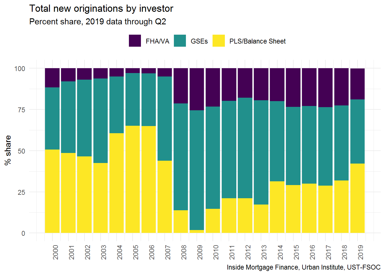

Total Homeowner Equity

Homeowner equity is an important metric in understanding wealth effects in the broader economy. There are two main components which drive this figure: (i) age of the mortgage (i.e. how many payments towards acquiring the asset as a homeowner made); (ii) home price valuations.

The data we’re utilizing is produced by the Federal Reserve (FRB) and is aggregated in what was previously known as their flow of funds reports, now “The Financial Accounts of the United States.” In further posts, we’ll explore homeowner equity at a more granular level.

For this analysis, we use the tidyquant package, which has a wrapper to easily serve update the data. I utilize this primarily for economic data, but it can also be utilized for stock market information. We will primarily be utilizing the function tidyquant:tq_get(), which is passed a symbol or ticker

We will get all the data at once to make our minimal pre-processing easier.

1. Create a vector of tickers/symbols OR a tibble for additional context
2. Use tidyquant::tq_get to retrieve data
3. Do some minor cleaning: (i) convert dates to quarters; (ii) create separated year and month values for future plotting

# Create tibble of Economic Data of Interest w/ Short Description

fred_base_url <- "https://fred.stlouisfed.org/series/"
d_tks <- tibble(tks = c("OEHRENWBSHNO", "HOEREPHRE", "MDOTP1T4FR", "GDP", 
                        "CCLBSHNO", "HHMSDODNS", "CMDEBT", "HNODPI"), 
                title = c("Households (HH); owners' equity in real estate, Level", 
                          "Households; owners' equity in real estate as a percentage of household real estate, Level", "Mortgage Debt Outstanding by Type of Property: One- to Four-Family Residences", "Gross Domestic Product, Seasonally Annual Adjusted Rate", 
                          "HH Consumer Credit", "HH Mortgage Debt", "HH Credit Market Instruments", "HH Disposable Personal Income"))%>%
  mutate(row_id = row_number(), 
         url = paste0(fred_base_url, tks))


# LOAD ALL TICKERS 
# **NOTE** WE WONT BE USING ALL OF THESE METRICS

# tq_get automatically gets a "shorter" time period so we define long-run time-series
# the function returns the date as a full yyyy-mm-dd given different variables are 
# reported at different frequency. We know these are all reported quarterly by the fed
# since they come from the same report


# Finally, tickers are great, be we'll join our reference tibble for future reproducibility 
# 
d_eco <- tidyquant::tq_get(x = d_tks$tks, get = "economic.data", from = "1975-01-01")%>%
  mutate(dt_qtr = case_when(
    month(date) == 1 ~ paste0(year(date), "-Q1"), 
    month(date) == 4 ~ paste0(year(date), "-Q2"), 
    month(date) == 7 ~ paste0(year(date), "-Q3"), 
    month(date) == 10 ~ paste0(year(date), "-Q4")
  ))%>%
  left_join(., select(d_tks, tks, title), by = c("symbol"="tks"))%>%
  rename(value = price)

d_hh_eq <- filter(d_eco, symbol == "HOEREPHRE")

p_hh_eq_curr <- d_hh_eq%>%
  slice(which.max(date))%>%
  mutate(clean_lab = paste0(dt_qtr, ": ", prettyNum(round(value,0), big.mark = ","), "%"))%>%
  select(date, value, clean_lab)

p1_hh_eq <- d_hh_eq%>%
  ggplot()+
  geom_line(aes(x = date, y = value), color = "navy", size = 1.15)+
  geom_hline(data = p_hh_eq_curr, aes(yintercept = value), color = "darkred", size = 1.1, linetype = 2)+
  geom_point(data = p_hh_eq_curr, aes(x = date, y = value), size = 5, color = "darkred", 
             alpha = 0.7)+
  scale_x_date(date_breaks = "3 years", date_labels = "%Y")+
  scale_y_continuous(labels = dollar)+
  labs(title = "Households (HH) homeowners equity as % of HH real estate", 
       subtitle = paste("As of", p_hh_eq_curr$clean_lab), 
       x = NULL,
       y = "%", 
       caption = "U.S. Federal Reserve Board (FRB)")+
  theme_minimal()

p1_hh_eq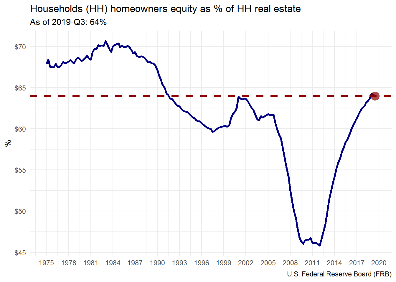

What next?

Those are just a few metrics, we’ll take a deeper dive in future posts as it relates to: (i) meaningfulness of the data; (ii) alternative metrics to compare against; (iii) components of aggregate measures and maybe even a function to quickly plot future FRB data…