About the Project
Each week The Economist shows up in my mailbox and I am met with the conflicting sentiment of excitement and despair. Excited to have the latest news with more reflection than the pace of twitter, but despair because I have normally only consumed one or two articles from the previous issue arriving.
Between work, other news sources and my appetite to continue to hone my skills in R – little time is left for consuming the dense and frequent writing. The solution, attempt to consolidate my hobbies, by selecting a chart from each issue to recreate with R!
Throughout 2018, I will try to re-create a single chart from each issue released throughout 2017 (did I mention, I can’t throw them away…) with the hope of catching up the more recent issues by half way through the year.
So let’s begin…
Magazine Details
January 2017 - Week 1
Issue Title: The Next Frontier
Article Title: Italy, Their Generation
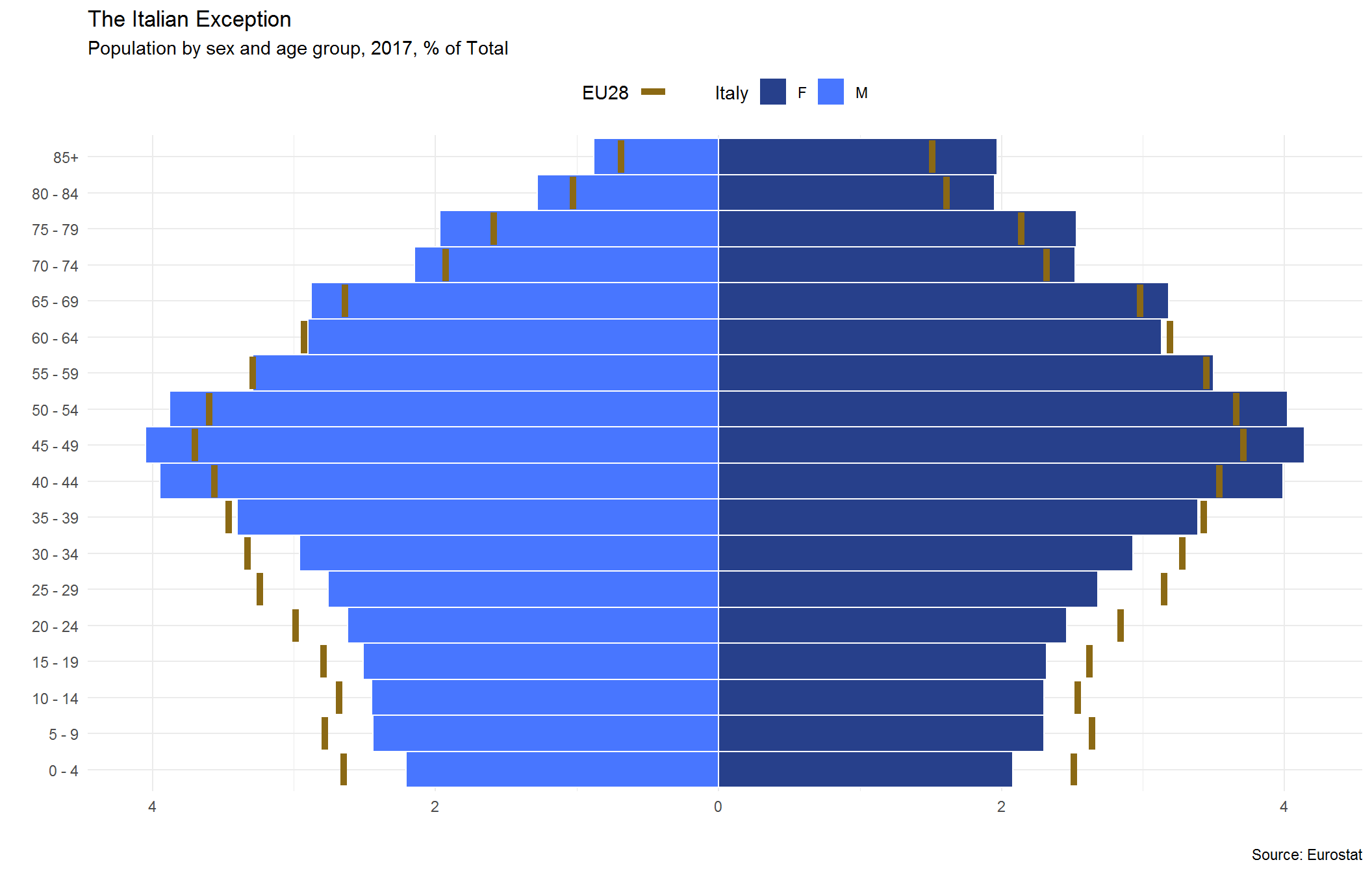
Graph Title: The Italian Exception
Article Page Number: 35
Data Details
Data Source: eurostat
Data Table Title: demo.pjan
Data Table Code: tps00001
Data Base Link: Here
Data Category: Demographics
About the Data
Admittedly, I did do some massaging of the data outside of R in order to get it into a better state for loading…I may or may never come back to do the cleaning in R or better yet, use the eurostat package to load the data directly.
# rm(list = ls())
# Optional - don't treat strings as factors,
# no scientific notation for large #'s
options(stringsAsFactors = F, scipen = 99)

# Required Packages - install if necessary
# UPDATE TO INSTALL IF DON'T EXISt
pks <- c("tidyverse", "purrr", "tools", "fs", "lubridate",
         "stringr", "readxl", "ggthemes", "eurostat")

invisible(lapply(pks, require, character.only = T))


# Name of the file for reading in
# NOTE - this may vary depending on your file names
d_fname <- "1.1_eu_pop_by_age.tsv"
Load Data and Clean it Up
Unfortunately, read_tsv does not import perfectly – so we need to do some additional cleaning:
Cleaning Steps
- Select columns of interest
- Separate columns that did not import correctly and rename
- Filter data to grab geographies of interest (Italy v. EU28 combined)
- Remove totals and unknown age observations
- Further clean-up observations
- Create age cohort groups (data is individual years/age)
Aggregating Steps
- Create clean labels by establishing a FROM age TO age
- Create an 85+ Category
- Get total population by Italy v. EU28 (for percent of total calc)
- Create totals and percent of total by additional groups (sex, age cohort)
- Ensure that one value (M = Negative, F = Positive) for our pyramid plot
# https://blogdown-demo.rbind.io/2018/02/27/r-file-paths/
# For reading in data with blogdown

## NOTE special directory for the data files

age_cut <- seq(0,85,5)

# Data loading and cleaning
d <- read_tsv(paste0("../../static/data/econ-viz-data/jan-issues/",
                     d_fname),
              col_names = T)%>%
  select(contains("unit"), `2017`)%>%
  separate(.,col = "unit,age,sex,geo\\time", sep=",", into = c("unit", "age", "sex", "geo"))%>%
  filter(geo %in% c("IT", "EU28"))%>%
  filter(!age %in% c("TOTAL", "UNK"))%>%
  filter(!sex == "T")%>%
  filter(age != "Y_LT1" , age !="Y_OPEN")%>%
  mutate(age = as.numeric(str_replace_all(age, pattern="Y", "")),
         value_2017 = as.numeric(str_replace_all(`2017`, pattern="[^0-9]", "")),
         age_cut = cut(age, breaks = c(seq(0,85,5), Inf)))%>%
  select(-`2017`)

# Data aggregations by groupings
d_sub <- d%>%
  separate(age_cut, sep = ",", into = c("from", "to"), remove = F)%>%
  mutate_at(vars("from", "to"), str_replace_all, pattern = "[^0-9]","")%>%
  mutate(to = as.numeric(to)-1)%>%
  mutate(clean_lab = paste0(from, " - ", as.character(to)),
         clean_lab = if_else(grepl(clean_lab, pattern = "NA")==T, "85+", clean_lab))%>%
  select(-c(unit, from, to))%>%
  group_by(geo)%>%
  mutate(tot_pop = sum(value_2017, na.rm = T))%>%
  group_by(sex, age_cut, clean_lab, add = T)%>%
  summarize(cohort_pop = sum(value_2017, na.rm = T),
            pct_tot = cohort_pop/unique(tot_pop))%>%
  mutate(plot_value_pct = if_else(sex=="M", round((pct_tot*-1)*100,2),
                                  round(pct_tot*100, 2)))%>%
  arrange(geo, age_cut)%>%
  ungroup()
Build Plot - Pyramid Plot
Pyramid plots are the most frequently utilized tool for evaluating demographic trends within a geography. Since population demographics are a massive contributor to economic measures (especially housing), it is important to know how much of the population is of prime working age, entering retirement or somewhere in between. Generally a younger population indicates pent up economic output that will be realized in the future, while a large aging population is more concerning since there will be less overall contribution to the economy (and sometimes even a drag depending on the social programs within the country – think healthcare as an example)
Since the Economist viz includes bars as the baseline to compare the Italy population against other EU28 countries, we will first extract a summary measure for that aggregation. Then we we can build our pyramid (barplot) and overlay where Italy sits by age cohort relative to the combined population of the EU28 cohorts by gender.
eu28_bar <- filter(d_sub, geo == "EU28") %>% select(age_cut, sex, plot_value_pct)

ggplot(data = filter(d_sub, geo == "IT") %>% arrange(geo, age_cut), aes(x = age_cut,
    y = plot_value_pct, fill = sex)) + geom_bar(stat = "identity", width = 1,
    color = "white") + geom_errorbar(data = filter(d_sub, geo == "EU28") %>%
    arrange(geo, age_cut), aes(ymax = plot_value_pct, ymin = plot_value_pct,
    color = "goldenrod4"), size = 1.85) + theme_minimal(base_family = "Roboto") +
    scale_y_continuous(breaks = c(seq(-10, 10, 2)), labels = function(y) paste0(abs(y))) +
    scale_x_discrete(labels = unique(d_sub$clean_lab)) + scale_fill_manual(name = "Italy",
    values = c("royalblue4", "royalblue1")) + scale_color_manual(name = "EU28",
    values = "goldenrod4", labels = NULL) + coord_flip() + labs(x = "", y = "",
    title = "The Italian Exception", subtitle = "Population by sex and age group, 2017, % of Total",
    fill = "", caption = "Source: Eurostat") + theme(legend.position = "top",
    legend.direction = "horizontal")