Freddie Mac Quarterly Re-Fi

Mortgage Statistics on Refinance Volume

This is a short post on gathering data from Freddie Mac based on their quarterly data published by Freddie Mac on volume of refinance transactions by refinance type.

Additional information about the institution and this particular dataset can be found on the company’s site (here)1.

The quarterly refinance statistics analysis uses a sample of properties where Freddie Mac has funded two successive conventional, first-mortgage loans, and the latest loan is for refinance rather than for purchase. The analysis does not track the use of funds made available from these refinances. The analysis also does not track loans paid off in entirety, with no new loan placed. Some loan products, such as 1-year adjustable-rate mortgages (ARMs) and balloons, are based on a small number of transactions.

Once we have the url of the most recently published dataset, we can generate a function to download the file and load it into R for visualization.

Create the Function & Set the URL for the Data

You can also embed plots, for example:

fre_refi_url <- "http://www.freddiemac.com/research/docs/q3_refinance_2018.xls"


# Function:
get_fre_qtr_refi <- function(fre_refi_url){
  
  fre_col_nms <- c("dt_qtr_yr", "cash_out_pct", "no_chng_pct", "lower_loan_amt_pct", 
                   "median_ratio_new_old", "median_age_refi", "median_hpa_refi", 
                   "dt_qtr_yr2")
  if(missing(fre_refi_url)){
    base_fre_refi_url <- "http://www.freddiemac.com/research/datasets/refinance-stats/"
    paste0("Find the most recent dataset here: ", base_fre_refi_url)
  }else{
    
    tf <- tempfile()
    download.file(fre_refi_url, tf, mode = "wb")
    file.rename(tf, paste0(tf, ".xls"))
    
    d_fre <- read_excel(paste0(tf, ".xls"), skip = 5, sheet = 1)%>%
      select(-contains("X_"))%>%
      setNames(., fre_col_nms)%>%
      na.omit()
    
    st_dt_yr <- str_sub(d_fre$dt_qtr_yr, 0, 4)%>%head(.,1)%>%as.numeric()
    st_dt_qtr <- str_sub(d_fre$dt_qtr_yr, -2)%>%
      head(.,1)%>%
      as.numeric()%>%
      ifelse(. == 1, ., (.*3)+1)
    
    end_dt_yr <- str_sub(d_fre$dt_qtr_yr, 0, 4)%>%tail(.,1)%>%as.numeric()
    end_dt_qtr <- str_sub(d_fre$dt_qtr_yr, -2)%>%
      tail(.,1)%>%
      as.numeric()%>%
      ifelse(. == 1, ., (.*3)+1)
    
    seq_dt <- seq(ymd(paste(st_dt_yr, st_dt_qtr, "01", collapse = "-")), 
                  ymd(paste(end_dt_yr, end_dt_qtr, "01", collapse = "-")), 
                  by = "quarter")%>%
      tail(., -1)
    
    d_fre <- d_fre%>%
      mutate(dt_full = seq_dt)
  }
  unlink(tf)
  return(d_fre)
}

Get Data Loaded and Make Transformations

Now that we have our function and url, lets: * Download the data with our function * The function also loads the data, removing unecessary columns * In addition, we setup our dates to be cleaner full dates (i.e. ymd) * Finally, we take some extra steps to setup a new “long” dataset for plotting + This requires us to gather the data + Create a refinance type factor variable that is ordered for plotting

d_refi <- get_fre_qtr_refi(fre_refi_url)

d_refi_long <- d_refi%>%
  select(dt_full, contains("pct"))%>%
  gather(refi_type, value, -dt_full)%>%
  mutate(refi_type_f = factor(refi_type, levels = rev(c("cash_out_pct","lower_loan_amt_pct", "no_chng_pct")), 
                              labels = rev(c("Cash-Out", "Lower Loan Amount", "No Change")), ordered = T))

Plot Data

Next we will make a quick plot with ggplot2 to see how the proportion of refinance types has changed over time.

ggplot(data = d_refi_long)+
  geom_area(aes(x = dt_full, y = value, fill = refi_type_f))+
  scale_y_continuous(label = percent)+
  scale_fill_manual(values = alpha(c("navyblue", "darkorange1", "seagreen"), 0.85), NULL)+
  labs(title = "Quarterly Refinance by Type", 
       subtitle = "Freddie Mac Re-Fi's Only", 
       x = NULL, 
       y = "Percent Type (%)", 
       caption = "Source: Freddie Mac")+
  theme_minimal()+
  theme(legend.position = "top")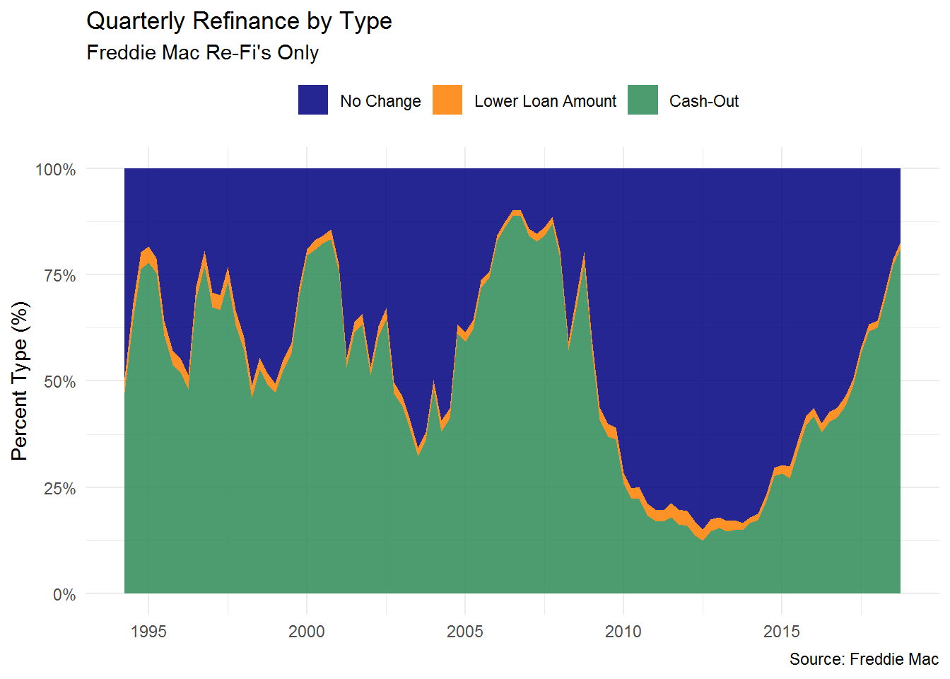

Notes & Plot Save

If we wanted to write the markdown file, html or save the plot we could do the following

# ggsave(filename = "Name-your-file.png", height = 7, width = 9, bg = "transparent")